Introduction

The problem of finding something is an important task. Many of us will spend countless hours in our lives looking for our keys or phone or trying to find the best tomatoes at the grocery store. In computer science, finding a specific record in a database can be an important task. Another common use for searching is to check if a value already exists in a collection. This function is important for implementing “sets” or collections of unique elements.

With the search problem, we start to think a little more about our data structures and what a solution means in the context of the data structure used. Suppose, for example, that we have an array of the following values using 0-based indexing.

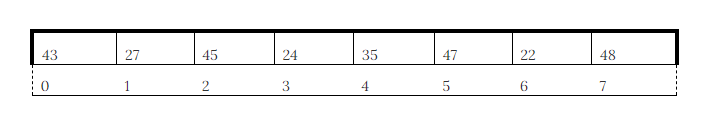
Figure 4.1

What does it mean to find the value 22? Should we return True if 22 is in the array? Should we return the index 6 instead? What should we do if 22 is not found? These questions will depend on how the search function is used in its broader context.

Let us describe a search problem in more detail. First, we are looking for a specific value or a record identified by a specific code in our data set. We will call the value for which we are searching the “key.” The key is a data value used to find a match in the data structure. For a simple array, the key is just the value itself. For example, 22 could be the key for which we are looking. Further, we may specify that our algorithms should return True if the key is found in our data structure and False if we fail to find the key. With our previous array, a call to search(array, 22) should return True, but a call to search(array, 12) should return False.

We now have an idea of what our search function should do, but we do not yet have an idea of how it should do it. Can you think of a way to implement search? Take a few minutes to think about it.

I am sure most computer science students would come to the same idea. Examine all the values of the array one by one, which is also known as iterating. If one of the values matches the key, return True. If we get to the end without finding the key, return False. This is a simple idea that will definitely work. This is the strategy behind Linear Search, which we will examine in the next section.

Linear Search

Linear Search may be the simplest searching algorithm. It uses an approach similar to the way a human might look for something in a systematic way—that is, by examining everything one by one. If your mother puts your clothes away and you are trying to find your favorite shirt, you might try every drawer in your room until it is found. Linear Search is an exhaustive search that will eventually examine every value in an array one by one. You can remember the name linear by thinking of it as going one by one in a line through all the values. Linear is also a clue that the runtime is O(n) because in the worst case, we must examine all n items in the array.

Let us examine one implementation of Linear Search.

Linear Search Complexity

As always, we will be interested in assessing the time and space scaling behavior of our algorithm. This means we want to know how its resource demand grows with larger inputs.

For space complexity, Linear Search needs storage for the array and a few other variables (the index of our for-loop, for example). This leads to a bound of O(n) space complexity.

For time complexity, we want to think about the best-case and worst-case scenarios. Suppose we go to search for the key, 22, and as luck would have it, 22 is the first value in the array! This leads to only a small number of operations and only 1 comparison operation. As you may have guessed, the best-case scenario leads to an O(1) or constant number of operations. In algorithm analysis (as in stock market investing), luck is not a strategy. We still need to consider the worst-case behavior of the algorithm, as this characteristic makes a better tool for evaluating one algorithm against another. In general, we cannot choose the problems we encounter, and our methods should be robust against all types of problems that are thrown at us. The worst case for Linear Search would be a problem where our key is found at the end of the array or isn’t found at all. For inputs with this feature, our time complexity bound is O(n).

Linear Search with Objects

Suppose we designed our Linear Search function to return the actual value of the key. For the array [43, 27, 45, 24, 35, 47, 22, 48], search(array, 22) would return 22. An important design consideration is this: What should it return if the value is not found in the array? Some approaches would return −1, but this would limit our search values to positive integers. What is needed is some type of sentinel value. This is another special value, unlike the ones we are storing. Another approach could be to throw an exception if the value is not found. There are many ways to address this problem, and this issue is an important one when storing more complex data types than just integers.

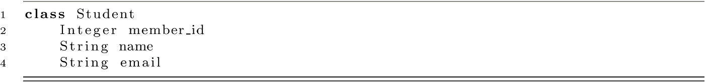
Suppose we are working on a database of contact information for a student club. We would design a class or data type specification for the student records that we need to store in our data structures. Our Student class might look something like the code below:

Now think about storing an array of Student object instances in memory. The diagram below is one way to visualize this data structure:

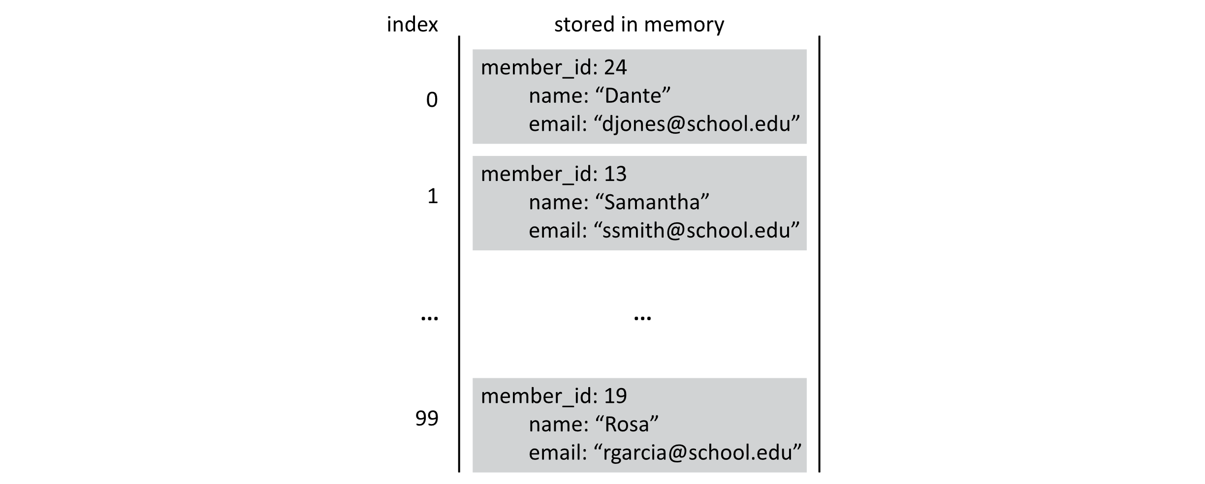
Figure 4.2

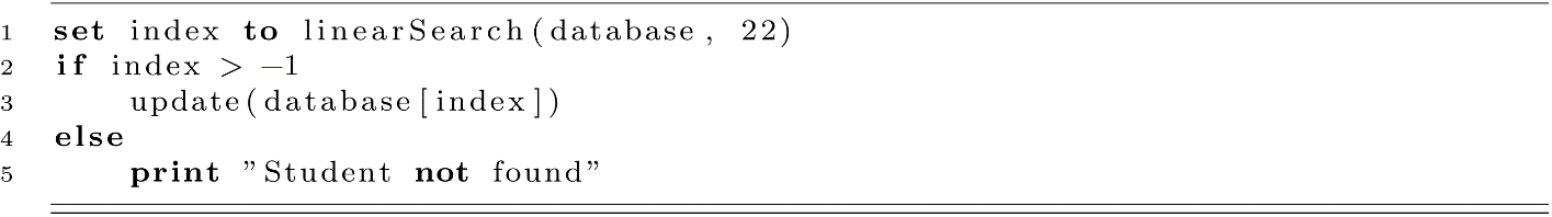
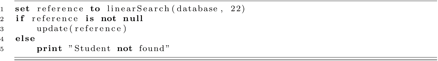
Now suppose we want to search through our database for the student whose member_id is 22. If our student is in the array, we could just return the Student object. If there is no student with 22 as their member_id, we run into the issues we mentioned above. All these issues create some difficulties in designing the interface of our search algorithm. A simple solution that could sidestep the problem would be to return either the index of the value or −1 to indicate that the value was not found. For many programming languages, −1 is an invalid array index.

Let us try our implementation of Linear Search one more time using the indexed approach and assume that our array holds a set of Student objects.

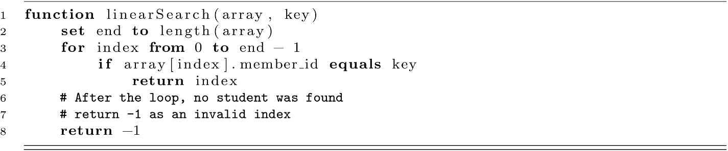
An example use of this implementation is given below. The programmer could access a student object safely (only if it was found) using the array index after the array has been searched.

A slight variation on this idea comes from a slightly altered database. Rather than storing all our student records in continuous blocks of memory, we may have an array of references to our records. This would lead to a structure like that depicted in the following image:

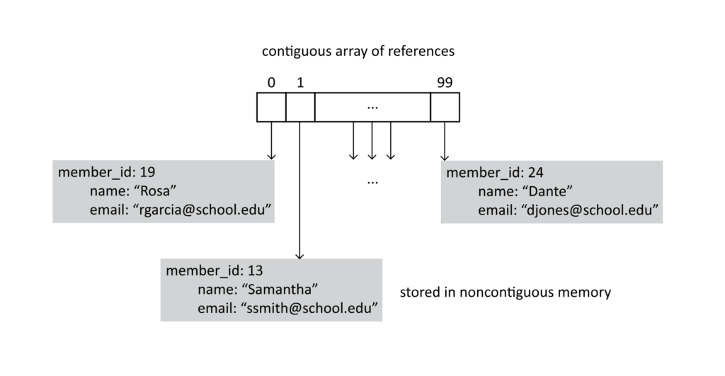
Figure 4.3

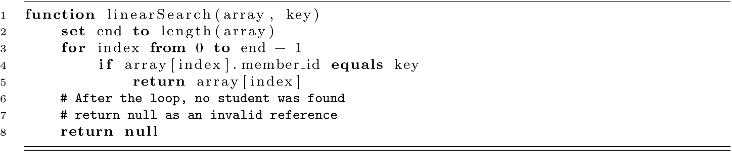
For this style of storage, our array holds references to instances rather than having the instances of objects stored in the array. Holding references rather than objects comes with some advantages in flexibility, but working with references puts more responsibility for memory management in the hands of the programmer. For the present search problem, working with references gives a nice solution to the “not found” problem. Specifically, we can return a null reference when our search fails to find an object with the matching search key.

Suppose now that our database of students is an array of references to objects. Our implementation would look like this:

Using this implementation as before may look something like this:

These examples will help you appreciate how simple design questions can lead to difficult issues when implementing your algorithm. Even without thinking about performance (in terms of Big-O complexity), design issues can impact the usability and usefulness of real-world software systems. Answering these design questions will inevitably impose constraints on how your algorithm can and will be used to solve problems in real-world contexts. It is important to carefully consider these questions and to understand how to think about answering them.

Binary Search

We have seen a method for searching for a particular item in an array that runs in O(n) time. Now we examine a classic algorithm to improve on this search time. The Binary Search algorithm improves on the runtime of Linear Search, but it requires one important stipulation. For Binary Search to work, the array items must be in a sorted order. This is an important requirement that is not cost-free. Remember from the previous chapter that the most efficient general-purpose sorting algorithms run in O(n log n) time. So you may ask, “Is Binary Search worth the trouble?” The answer is yes! Well, it depends, but generally speaking, yes! We will return to the analysis of Binary Search after we have described the algorithm.

The logic of Binary Search is related to the strategy of playing a number-guessing game. You may have played a version of this game as a kid. The first player chooses a number between 1 and 100, and the second player tries to guess the number. The guesser guesses a number, and the chooser reports one of the following three scenarios:

1. The guesser guessed the chooser’s number and wins the game.
2. The chooser’s number is higher than the guess, and the chooser replies, “My number is higher.”
3. The chooser’s number is lower than the guess, and the chooser replies, “My number is lower.”

An example dialogue for this game might go like this:

Chooser: [chooses 37 in secret] “I have my number.”

Guesser: “Is your number 78?”

Chooser: “My number is lower.”

Guesser: “Is your number 30?”

Chooser: “My number is higher.”

Guesser: “Is your number 47?”

Chooser: “My number is lower.”

Guesser: “Is your number 35?”

Chooser: “My number is higher.”

Guesser: “Is your number 40?”

Chooser: “My number is lower.”

Guesser: “Is your number 38?”

Chooser: “My number is lower.”

Guesser: “Is your number 37?”

Chooser: “You guessed my number, 37!”

With each guess, the guesser narrows down the possible range for the chooser’s number. In this case, it took 7 guesses, but if the guesser is truly guessing at random, it could take much longer. Where does Binary Search come in? Well, take a few moments to think about a better strategy for finding the right number. When the guesser guesses 78 and the chooser responds with “lower,” all values from 78 to 100 can be eliminated as possibilities. What strategy would maximize the number that we eliminate each time? Maybe you have thought of the strategy by now.

The optimal strategy would be to start with 50, which eliminates half of the numbers with one guess. If the chooser responds “lower,” the next guess should be 25, which again halves the number of possible guesses. This process continues to split the remaining values in half each time. This is the principle behind Binary Search, and the “binary” name refers to the binary split of the candidate values. This strategy works because the numbers from 1 to 100 have a natural order.

A precondition for Binary Search is that the elements of the array are sorted. The sorting allows each comparison in the array to be oriented, and it indicates in which direction to continue the search. Each check adds some new information for our algorithm and allows the calculation to proceed efficiently.

We will present an illustration below of an example execution of the algorithm. Suppose we are searching for the key 27 in the sorted array below:

Figure 4.4

We will keep track of three index variables to track the low and high ends of the range as well as a “mid” or middle variable that will track the middle value in the range. The mid variable will be the one currently considered for the key. In this case, 35 is too high, so we will update the high end of the range. The high variable will be set to mid − 1, and we will recalculate the mid.

Figure 4.5

At this point in the execution, mid at 1 means we are considering the value 24. As 27 is greater than 24, we will now update the low variable to mid + 1 or 2.

Next, we have the case where low equals high, and that means either we have found the key or the key does not exist. We see that 27 is in the array, and we would report that it is found. The image below gives this scenario:

Figure 4.6

The game description and array example should give you an idea of how Binary Search can efficiently find keys in a sorted data structure. Let us examine an implementation of this algorithm. For our design, we will return the index of the value if it is found or −1 as an invalid index to indicate the key was not found. We will consider an array of integer keys, but it will work equally well with objects assuming they are sorted by their relevant keys.

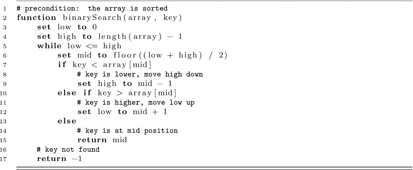
This is a subtle and powerful algorithm. It may take some thinking to understand. Think about when the algorithm would reach line 15. This means that the value at array[mid] is neither higher nor lower than the key. If it is not higher or lower, it must be the key! We return the index of the key in this case.

The case of the key missing from the array is also subtle. How could the algorithm reach line 17? To reach line 17, low must be a value greater than high. How could this happen? Think back to our example above when low, high, and mid were all pointing to index 2 and we were searching for the key 27. Suppose instead of 27 at position 2, the array had 25 at position 2, which still preserved the sorted order (22, 24, 25, 35, 43, 45, 47, 48). The algorithm would check “Is 27 less than 25?” at line 7. No, this is false. Next, it would check “Is 27 greater than 7?” at line 10. This is true, so low would be updated to mid + 1, or 3 in this case, and the loop would begin again. Only now, low is 3 and high is 2, and the loop condition fails and the return −1 at line 17 is reached.

Binary Search Complexity

Now we will assess the complexity of Binary Search. The space complexity of Binary Search is O(1) or constant space. From another perspective, one might consider this auxiliary space and say that O(n) space is needed to hold the data. From our perspective, we will assume that the database is needed already for other purposes and not consider its O(n) space cost a requirement of Binary Search. We will only consider the space demand for the algorithm to be the few extra variables that serve as the array indexes. Specifically, our algorithm only uses the low, high, and mid indexes. We could also factor in a reference for the array’s position in memory and a copy of the key value. Even with these extra variables consuming space, only a constant amount of extra memory is needed, leaving the space complexity of the array-based Binary Search at O(1).

The time complexity of Binary Search requires a bit of explanation, but the logic behind the proof is similar to arguments we have seen before (see “Powers of 2 in O(log n) Time” in chapter 2 and “Merge Sort Complexity” in chapter 3). First, consider the best-case scenario. The best case would be if the key item is found at the mid position on the very first check. In our example above, this would occur if our key was 35, which is in position 3 (mid = floor((0 + 7) / 2) = 3). In the best case, the time complexity of Binary Search is O(1). This matches the best case for Linear Search. In the worst case, Binary Search must continue to update the range of possible locations for the key. This update process essentially eliminates half of the range each time our loop runs. This means that determining the Big-O complexity for Binary Search depends on determining how many times we can halve the range before reaching a single element. Here we have repeated division by two, which we should now know leads to O(log n). We will present this a little more formally below. Letting T(n) be the time cost in the number of operations for Binary Search on an array of N elements,

Here c is a constant number of operations (making a comparison, updating a value, and so on; it may be different on different computer architectures).

We can expand this like so:

This leads us to the following formula:

Ultimately, repeatedly reducing the range of valid choices will lead to a single element that must be compared with the key. So we want to find the k that makes n/2^k equal to 1. This value is log₂ n, which we will abbreviate to just log n.

Substituting back into the equation gives the following:

We are left with a constant multiple of log n for a worst-case time complexity of O(log n).

A time complexity of O(log n) is considered extremely fast in most contexts and is an excellent scaling bound for an algorithm. Consider a Linear Search with 1,000 items. That algorithm may have to make nearly 1,000 comparison checks to determine if the key is found. A Binary Search for a sorted array of 1,000 items needs to make only about 10 checks. For an array of 1,000,000 elements, the Linear algorithm may make nearly 1 million checks, while the Binary Search checks only about 20 in the worst case! That is an excellent improvement (1 million >> 20).

Binary Search Complexity in Context

We are all ready to celebrate and embrace the amazing properties of Binary Search with its O(log n) search time complexity, but there is a catch. As we mentioned, the array must be sorted, and typically we cannot do much better than O(n log n) for sorting (without some extra information). Would that mean that, in reality, Binary Search is O(n log n + log n) leading to O(n log n)? In a sense, yes. If we had to start from an unsorted array, we would need to first sort it. This would give us a sorting cost of O(n log n). Then any subsequent search on the data would only cost O(log n). This would make the total cost of Binary Search bounded by its most expensive operation, the sorting part. Oh no, Binary Search is actually O(n log n)—all is lost! Well, let us use our analysis skills to try to determine why and when Binary Search would be more useful than Linear Search.

The important realization is that sorting is a one-time cost. Once the array is sorted, all subsequent searches can be done in O(log n). Let us think about how this compares to Linear Search, which always has a cost of O(n) regardless of the number of the number of times the array is searched. Another name for the act of searching is called a query. A query is a question, and we are asking the data structure the question “Do you have the information we need?” Suppose that the variable Q is the number of queries that are made of the data structure.

Querying our array using Linear Search Q times would give the following time cost with c being a constant associated with O(n):

Querying our array using Binary Search Q times would give the following cost:

Now suppose that Q was close to the size of n. We could rewrite these like this:

This leads to a time complexity of O(n²) for searching with approximately n different queries.

For Binary Search, we have the following adjusted formula:

This leads to a time complexity of O(n log n) for searching with approximately n different queries.

This means that if you plan on searching the data structure n or more times, Binary Search is the clear winner in terms of scalability.

As a final note, you should always try to run empirical tests on your workloads and hardware to draw conclusions about performance. Processor implementations on modern computers can further complicate these questions. For example, the CPU’s branch prediction and cache behavior may make Linear Search on a sorted list faster than some clever algorithmic search implementation in terms of actual runtimes.

References

Due to the age and simplicity of these algorithms, many of the published works in the early days of computing refer to them as being “well known.” Donald Knuth gives some early references to their origin in volume 3 of The Art of Computer Programming.
Knuth, Donald E. The Art of Computer Programming. Pearson Education, 1997.