Introduction

Recursion is a powerful tool for computation that often saves the programmer considerable work. As you will see, the benefit of recursion lies in its ability to simplify the code of algorithms, but first we want to better understand recursion. Let’s look at a simple nonrecursive function to calculate the product of 2 times a nonnegative integer, n, by repeated addition:

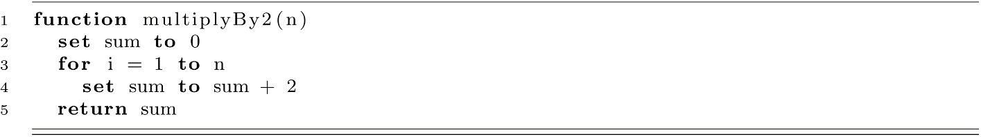
This function takes a number, n, as an input parameter and then defines a procedure to repeatedly add 2 to a sum. This approach to calculation uses a for-loop explicitly. Such an approach is sometimes referred to as an iterative process. This means that the calculation repeatedly modifies a fixed number of variables that change the current “state” of the calculation. Each pass of the loop updates these state variables, and they evolve toward the correct value. Imagine how this process will evolve as a computer executes the function call multiplyBy2(3). A “call” asks the computer to evaluate the function by executing its code.

When the process starts, sum is 0. Then the process iteratively adds 2 to the sum. The process generated is equivalent to the mathematical expression (2 + 2 + 2). The following table shows the value of each variable (i, sum, and n) at each time step:

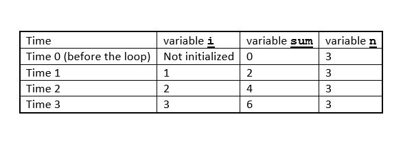
Figure 2.1

Recursive Multiplication

Like iterative procedures, recursive procedures are a means to repeat certain operations in code. We will now write a recursive function to calculate the multiplication by 2 as a sequence of addition operations.

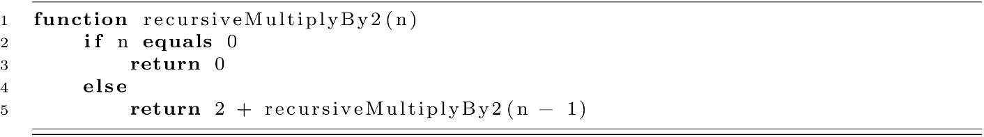
The recursive formulation follows the mathematical intuition that 2 * n = 2 + 2 * (n − 1) = 2 + 2 + 2 * (n − 2) … and so on until you reach 2 + 2 + 2 + … 2 * 1. We can visualize this process by considering how a computer might evaluate the function call recursiveMultiplyBy2(3). The evaluation process is similar conceptually to a rewriting process.

recursiveMultiplyBy2(3) -> 2 + recursiveMultiplyBy2(2)

-> 2 + 2 + recursiveMultiplyBy2(1)

-> 2 + 2 + 2 + recursiveMultiplyBy2(0)

-> 2 + 2 + 2 + 0

-> 2 + 2 + 2

-> 6

This example demonstrates a few features of a recursive procedure. Perhaps the most recognizable feature is that it makes a call to itself. We can see that recursiveMultiplyBy2 makes a call to recursiveMultiplyBy2 in the else part of the procedure. As an informal definition, a recursive procedure is one that calls to itself (either directly or indirectly). Another feature of this recursive procedure is that the action of the process is broken into two parts. The first part directs the procedure to return 0 when the input, n, is equal to 0. The second part addresses the other case where n is not 0. We now have some understanding of the features of all recursive procedures.

Features of Recursive Procedures

• A recursive procedure makes reference to itself as a procedure. This self-call is known as the recursive call.
• Recursive procedures divide work into two cases based on the value of their inputs.
  • One case is known as the base case.
  • The other case is known as the recursive case or sometimes the general case.

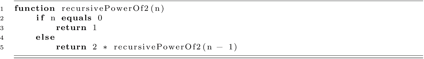
Recursive Exponentiation

Let us now consider another example. Just as multiplication can be modeled as repeated addition, exponentiation can be modeled as repeated multiplication. Suppose we wanted to modify our iterative procedure for multiplying by 2 to create an iterative procedure for calculating powers of 2 for any nonnegative integer n. How might we modify our procedure? We might simply change the operation from + (add) to * (multiply).

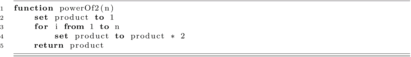
This procedure calculates a power of 2 for any nonnegative integer n. We changed not only the operation but also the starting value from 0 to 1.

We can also write this procedure recursively, but first let us think about how to formulate this mathematically by looking at an example. Suppose we want to calculate 2³:

The explicit 2⁰ is shown to help us think about the recursive and base cases. From this example, we can formulate two general rules about exponentiation using 2 as the base:

Now let’s write the recursive procedure for this function. Try to write this on your own before looking at the solution.

The Structure of Recursive Algorithms

As mentioned above, recursive procedures have a certain structure that relies on self-reference and splitting the input into cases based on its value. Here we will discuss the structure of recursive procedures and give some background on the motivation for recursion.

Before we begin, recall from chapter 1 that a procedure can be thought of as a specific implementation of an algorithm. While these are indeed two separate concepts, they can often be used interchangeably when considering pseudocode. This is because the use of an algorithm in practice should be made as simple as possible. Often this is accomplished by wrapping the algorithm in a simple procedure. This design simplifies the interface, allowing the programmer to easily use the algorithm in some other software context such as a program or application. In this chapter, you can treat algorithm and procedure as the same idea.

Some Background on Recursion

The concept of recursion originated in the realm of mathematics. It was found that some interesting mathematical sequences could be defined in terms of themselves, which greatly simplified their definitions. Take for example the Fibonacci sequence:

This sequence is likely familiar to you. The sequence starts at 0, 0 is followed by 1, and each subsequent value in the sequence is derived from the previous two elements in the sequence. This seemingly simple sequence is fairly difficult to define in an explicit way. Let’s look a bit closer.

Based on the sequence above, we see the following equations are true:

Using this formulation, we may wish to find a function that would calculate the nth Fibonacci number given any positive integer, n:

Finding such a function that depends only on n is not trivial. This also leads to some difficulties in formally defining the sequence. To partially address this issue, we can use a recursive definition. This allows the sequence to be specified using a set of simple rules that are self-referential in nature. These recursive rules are referred to in mathematics as recurrence relations. Let’s look at the recurrence relation for the Fibonacci sequence:

This gives a simple and perfectly correct definition of the sequence, and we can calculate the nth Fibonacci number for any positive integer n. Suppose we wish to calculate the eighth Fibonacci number. We can apply the definition and then repeatedly apply it until we reach the F₀ and F₁ cases that are explicitly defined:

This may be a long process if we are doing this by hand. This could be an especially long process if we fail to notice that F₇₋₂ is the same as F₆₋₁.

A Trade-Off with Recursion

Observing this process leads us to another critical insight about recursive processes. What may be simple to describe may not be efficient to calculate. This is one of the major drawbacks of recursion in computing. You may be able to easily specify a correct algorithm using recursion in your code, but that implementation may be wildly inefficient. Recursive algorithms can usually be rewritten to be more efficient. Unfortunately, the efficiency of the implementation comes with the cost of losing the simplicity of the recursive code. Sacrificing simplicity leads to a more difficult implementation. Difficult implementations allow for more bugs.

An Aside on Navigating the Efficiency-Simplicity Trade-Off

In considering the trade-off between efficiency and simplicity, context is important, and there is no “right” answer. A good guideline is to focus on correct implementations first and optimize when there is a problem (verified by empirical tests). Donald Knuth references Tony Hoare as saying “premature optimization is the root of all evil” in programming. This should not be used as an excuse to write inefficient code. It takes time to write efficient code. “I was optimizing the code” is a poor excuse for missed deadlines. Make sure the payoff justifies the effort.

Recursive Structure

The recursive definition of the Fibonacci sequence can be divided into two parts. The first two equations establish the first two values of the sequence explicitly by definition for n = 0 and n = 1. The last equation defines Fibonacci values in the general case for any integer n > 1. The last equation uses recursion to simplify the general case. Let’s rewrite this definition and label the different parts.

Base Cases

Recursive Case

Recursive algorithms have a similar structure. A recursive procedure is designed using the base case (or base cases) and a recursive case. The base cases may be used to explicitly define the output of a calculation, or they may be used to signal the end of a recursive process and stop the repeated execution of a procedure. The recursive case makes a call to the function itself to solve a portion of the original problem. This is the general structure of a recursive algorithm. Let’s use these ideas to formulate a simple algorithm to calculate the nth Fibonacci number. Before we begin, let’s write the cases we need to consider.

Base Cases

Recursive Case

Now we define the recursive algorithm to calculate the nth Fibonacci number.

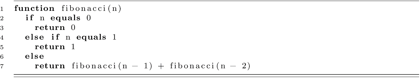
In this algorithm, conditional if-statements are used to select the appropriate action based on the input value of n. If the value is 0 or 1, the input is handled by a base case, and the function directly returns the appropriate value. If another integer is input, the recursive case handles the calculation, and two more calls to the procedure are executed. You may be thinking, “Wait, for every function call, it calls itself two more times? That doesn’t sound efficient.” You would be right. This is not an efficient way to calculate the Fibonacci numbers. We will revisit this idea in more detail later in the chapter.

Before we move on, let us revisit the two examples from the introduction, multiplication and exponentiation. We can define these concepts using recurrence relations too. We will use the generic letter a for these definitions.

Multiplication by 2

Base Case

Recursive Case

Powers of 2

Base Case

Recursive Case

Looking back at the recursive functions for these algorithms, we see they have a shared structure that uses conditionals to select the correct case based on the input, and the base cases and recursive cases handle the calculation by ending the chain of recursive calls or by adding to the chain of calls respectively. In the next section, we will examine some important details of how a computer executes these function definitions as dynamic processes to generate the correct result of a calculation.

Recursion and the Runtime Stack

Thus far, we have relied on your intuitive understanding of how a computer executes function calls. Unless you have taken a computer organization or assembly language course, this process may seem a little mysterious. How does the computer execute the same procedure and distinguish the call to recursiveMultiplyBy2(3) from the call to recursiveMultiplyBy2(2) that arises from the previous function call? Both calls utilize the same definition, but one has the value 3 bound to n and the other has the value 2 bound to n. Furthermore, the result of recursiveMultiplyBy2(2) is needed by the call to recursiveMultiplyBy2(3) before a value may be returned. This requires that a separate value of n needs to be stored in memory for each execution of the function during the evaluation process. Most modern computing systems utilize what is known as a runtime stack to solve this problem.

A stack is a simple data structure where data are placed on the top and removed from the top. Like a stack of books, to get to a book in the middle, one must first remove the books on top. We will address stacks in more detail in a later chapter, but we will briefly introduce the topic. Here we will examine how a runtime stack is used to store the necessary data for the execution of a recursive evaluation process.

The Runtime Stack

We will give a rough description of the runtime stack. This should be taken as a cartoon version or caricature of the actual runtime stack. We encourage you to supplement your understanding of this topic by exploring some resources on computer organization and assembly language. The real-world details of computer systems can be as important as the abstract view presented here.

The runtime stack is a section of memory that stores data associated with the dynamic execution of many function calls. When a function is called at runtime, all the data associated with that function call, including input arguments and locally defined variables, are placed on the stack. This is known as “pushing” to the stack. The data that was pushed onto the stack represents the state of the function call as it is executing. You can think of this as the function’s local environment during execution. We call this data stored on the stack a stack frame. The stack frame is a contiguous section of the stack that is associated with a specific call to a procedure. There may be many separate stack frames for the same procedure. This is the case with recursion, where the same function is called many times with distinct inputs.

Once the execution of a function completes, its data are no longer needed. At the time of completion, the function’s data are removed from the top of the stack or “popped.” Popping data from the runtime stack frees it, in a sense, and allows that memory to be used for other function calls that may happen later in the program execution. As the final two steps in the execution of the procedure, the function’s stack frame is popped, and its return value (if the function returns a value) is passed to the caller of the function. The calling function may be a “main” procedure that is driving the program, or it may be another call to the same function as in recursion. This allows the calling function to proceed with its execution. Let’s trace a simple recursive algorithm to better understand this process.

A Trace of a Simple Recursive Call

Suppose we are running a program that makes a call to recursiveMultiplyBy2(3). Consider the simple program below.

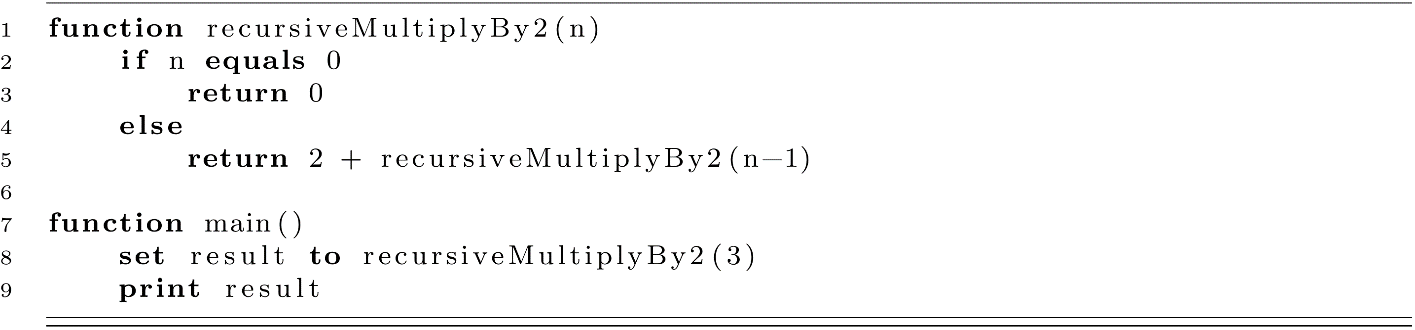
The computer executes programs in a step-by-step manner, executing one instruction after another. In this example, suppose that the computer begins execution on line 8 at the start of the main procedure. As main needs space to store the resulting value, we can imagine that a place has been reserved for main’s result variable and that it is stored on the stack. The following figure shows the stack at the time just before the function is called on line 8.

Figure 2.2

When the program reaches our call to recursiveMultiplyBy2(3), the n variable for this call is bound with the 3 value, and these data are pushed onto the stack. The figure below gives the state of the stack just before the first line of our procedure begins execution.

Figure 2.3

Here the value of 3 is bound to n and the execution continues line by line. As this n is not 0, the execution would continue to line 5, where another recursive call is made to recursiveMultiplyBy2(2). This would push another stack frame onto the stack with 2 bound to n. This is shown in the following figure.

Figure 2.4

You can imagine this process continuing until we reach a call that would be handled by the base case of our recursive algorithm. The base case of the algorithm acts as a signal that ends the recursion. This state is shown in the following figure:

Figure 2.5

Next, the process of completing the calculation begins. The resulting value is returned, and the last stack frame is popped from the top of the stack.

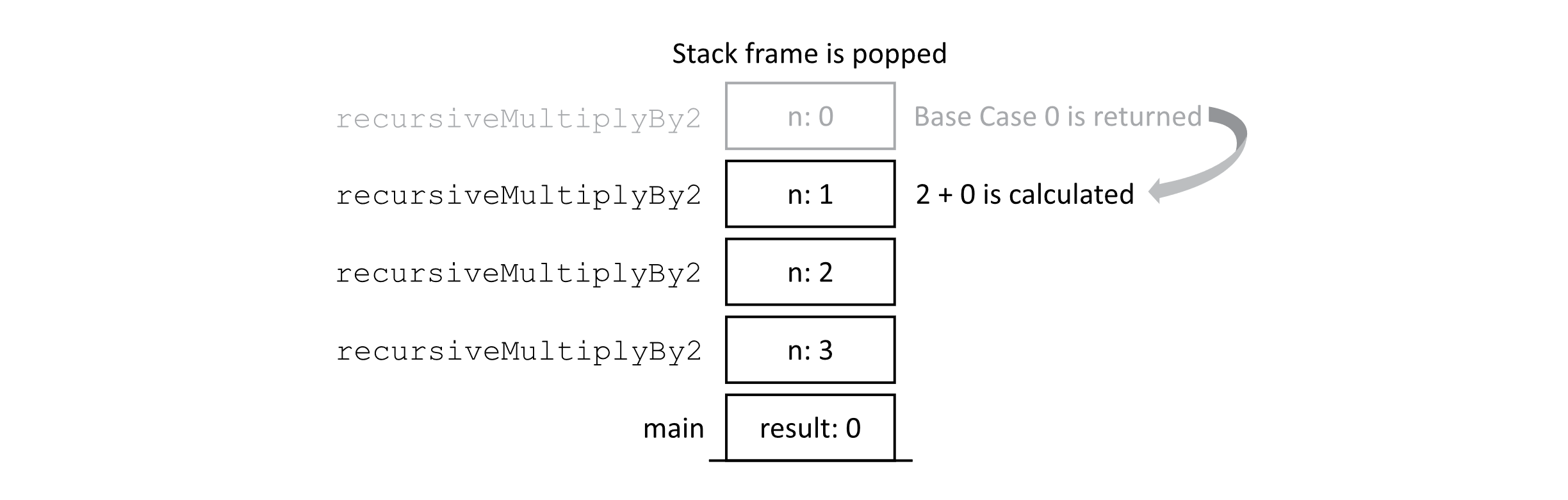
Figure 2.6

Once the call for n = 0 gets the returned value of 0, it may then complete its execution of line 5. This triggers the next pop from the stack, and the value of 2 + 0 = 2 is returned to the prior call with n = 2. Let’s look at the stack again.

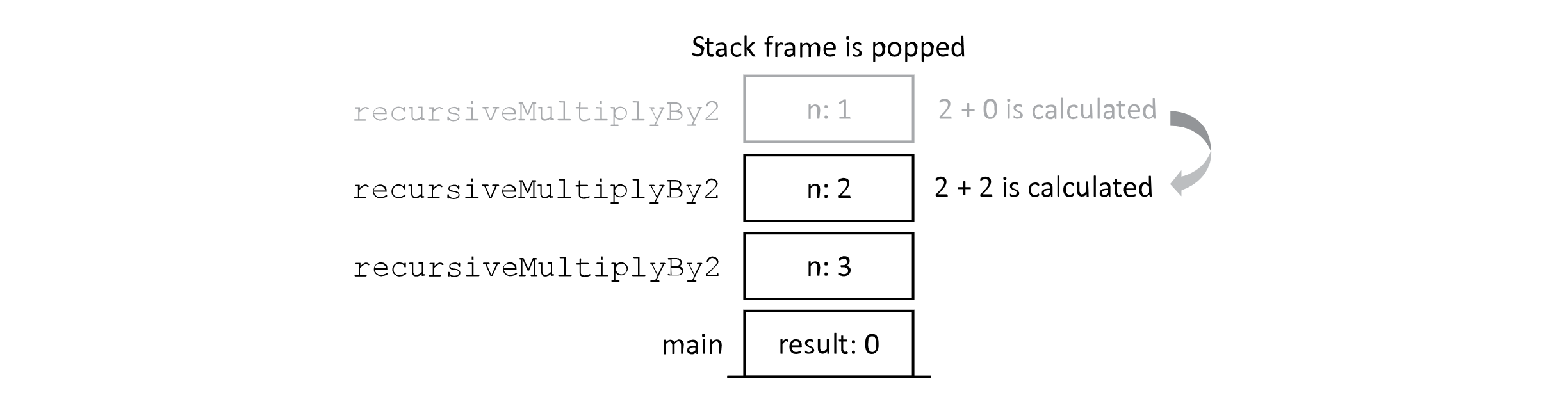
Figure 2.7

As we can see, the chain of calls is unwinding as the results are calculated in turn. This process continues. As the results are calculated and stack frames are popped, it should be clear that less memory is being used by the program. It should be noted that this implies a memory cost for deep chains of recursion. Finally, the last recursive call completes its line 5, and the value is returned to the main function as shown below.

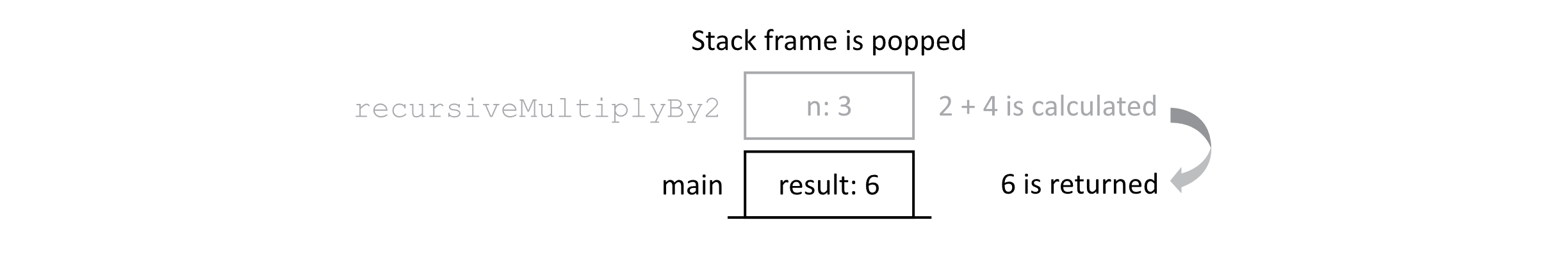
Figure 2.8

Now the main function has the result of our recursive algorithms. The value 6 is bound to the “result” variable, and when the program executes the print command, “6” would appear on the screen. This concludes our trace of the dynamic execution of our program.

Why Do We Need to Understand the Runtime Stack?

You may now be thinking, “This seems like a lot of detail. Why do we need to know all this stuff?” There are two main reasons why we want you to better understand the runtime stack. First, it should be noted that function calls are not free. There is overhead involved in making a call to a procedure. This involves copying data to the stack, which takes time. The second concern is that making function calls, especially recursive calls, consumes memory. Understanding how algorithms consume the precious resources of time and space is fundamental to understanding computer science. We need to understand how the runtime stack works to be able to effectively reason about memory usage of our recursive algorithms.

More Examples of Recursive Algorithms

We have already encountered some examples of recursive algorithms in this chapter. Now we will discuss a few more to understand their power.

Recursive Reverse

Suppose you are given the text string “HELLO,” and we wish to print its letters in reverse order. We can construct a recursive algorithm that prints a specific letter in the string after calling the algorithm again on the next position. Before we dive into this algorithm, let’s explain a few conventions that we will use.

First, we will treat strings as lists or arrays of characters. Characters are any symbols such as letters, numbers, or other type symbols like “*,” “+,” or “&.” Saying they are lists or arrays means that we can access distinct positions of a string using an index. For example, let message be a string variable, and let its value be “HELLO.” If we access the elements of this array using zero-based indexing, then message[0] is the first letter of the string, or “H.” We will be using zero-based indexing (or 0-based indexing) in this textbook. Switching between 0-based and 1-based indexing should be easy, although it can be tricky and requires some thought when converting complex algorithms. Next, saying that a string is an array is incorrect in most programming languages. An array is specifically a fixed-size, contiguous block of memory designed to store multiple values of the same type. Most programming languages provide a string type that is more robust. Strings are usually represented as data structures that provide more functionality than just a block of memory. We will treat strings as a data structure that is like an array with a little more functionality. For example, we will assume that the functionality exists to determine the size of a string from its variable in constant time or O(1). Specifically, we will use the following function.

Back to the algorithm, we will define the base and recursive cases. The base case that terminates the algorithm will be reached by the algorithm when the position to print is greater than or equal to the length of the string. The recursive case will call the algorithm for the next position and then print the letter at the current position after the recursive call.

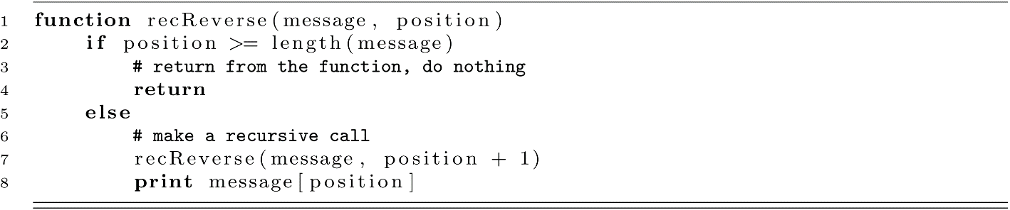
Calling recReverse(“HELLO”, 0) should give the following text printed to the screen:

O

L

L

E

H

This demonstrates that the recursive algorithm can print the characters of a string in reverse order without using excessive index manipulation. Notice the order of the print statement and the recursive call. If the order of lines 7 and 8 were switched, the characters would print in their normal order. This algorithm resembles another recursive algorithm for visiting the nodes of a tree data structure that you will see in a later chapter.

Wrappers and Helper Functions for Recursion

You may have noticed that recReverse(“HELLO”, 0) seems like an odd interface for a function that reverses a string. There is an extra piece of state, the value 0, that is needed anytime we want to reverse something. Starting the reverse process in the middle of the string at index 3, for example, seems like an uncommon use case. In general, we would expect that reversing the string will almost always be done for the entire string. To address this problem, we will make a helper function. Let’s create this helper function so we can call the reverse function without giving the 0 value.

Now we may call reverse(“HELLO”), which in turn, makes a call that is equivalent to revReverse(“HELLO”, 0). This design method is sometimes called wrapping. The recursive algorithm is wrapped in a function that simplifies the interface to the recursive algorithm. This is a very common pattern for dealing with recursive algorithms that need to carry some state of the calculation as input parameters. Some programmers may call reverse the wrapper and recReverse the helper. If your language supports access specifiers like “public” and “private,” you should make the wrapper a “public” function and restrict the helper function by making it “private.” This practice prevents programmers from accidentally mishandling the index by restricting the use of the helper function.

Greatest Common Divisor

An algorithm for the greatest common divisor (GCD) of two integers can be formulated recursively. Suppose we have the fraction 16/28. To simplify this fraction to 4/7, we need to find the GCD of 16 and 28. The method known as Euclid’s algorithm solves this problem by dividing two numbers, taking their remainder after division, and repeating the division step with one of the numbers and the remainder. Given two integers a and b, the algorithm proceeds according to this general process:

1. Take two integers a and b, and let a be larger than b.
2. Find the remainder of a / b, and let that number be r.
3. If r is 0, b is the GCD; otherwise, repeat the process with b and r in place of a and b in step 1.

The equations below illustrate this process. Here, let a equal 28, and let b equal 16:

For the fraction 16/28, dividing the denominator and the numerator by 4 gives the simplified fraction 4/7. This is illustrated below:

Before we start writing the algorithm, let us think about the base case and the recursive case. What signals the end of recursion? If the remainder of a divided by b is zero, this means that b is the greatest common divisor. This should be our base case. With any other inputs, the algorithm should make a recursive call with updated inputs. Let us examine one way to implement this algorithm. We will use the keyword mod to mean the remainder of two integers. For example, we will take the expression 7 mod 3 to be evaluated to the value 1. The keyword mod is a shortened version of the word “modulo,” which is the operation that calculates integer remainders after division.

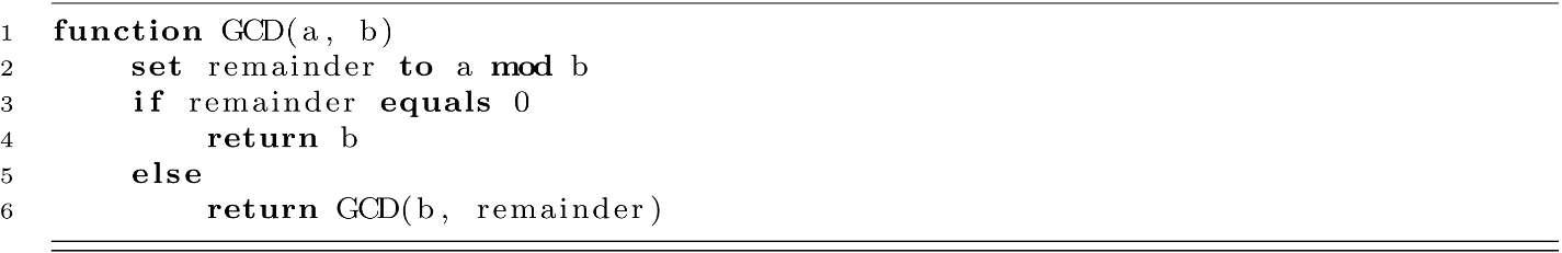
This process will continue to reduce a and b in sequence until the remainder is 0, ultimately finding the greatest common divisor. This provides a good example of a recursive numerical algorithm that has a practical use, which is for simplifying fractions.

Recursive Find Minimum

Finding the minimum value in a collection of numbers can be formulated as a recursive algorithm. Let us use an array of integers for this algorithm. Our algorithm will use the helper and wrapper pattern, and it will use an extra parameter to keep track of the current minimum value. Let us begin by specifying the core algorithm as a helper function. Here, as in recReverse, we assume a length function can provide the length of the array:

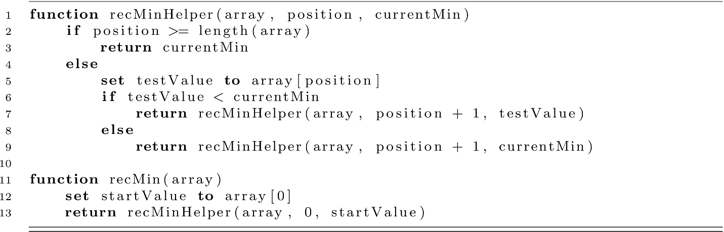
For this algorithm, our base case occurs when the recursive process reaches the last position of the array. This signals the end of recursion, and the currentMin value is returned. In the recursive case, we compare the value of the current minimum with the value at the current position. Next, a recursive call is made that uses the appropriate current minimum and increases the position.

Recursive Algorithms and Complexity Analysis

Now that we have a better understanding of recursive algorithms, how can their complexity be evaluated? Computational complexity is usually evaluated in terms of time complexity and space complexity. How does the algorithm behave when the size of the input grows arbitrarily large with respect to runtime and memory space usage? Answering these questions may be a little different for recursive algorithms than for some other algorithms you may have seen.

A Warm-Up, Nonrecursive Example: Powers of 2

Let us begin with the nonrecursive power-of-2 algorithm from the beginning of the chapter reprinted here:

For this algorithm, we observe a loop that starts at 1 and continues to n. This means that we have a number of steps roughly equal to n. This is a good clue that the time complexity is linear or O(n). For an n equal to 6, we could expand this procedure to the following sequence of 5 multiplications: 2 * 2 * 2 * 2 * 2 * 2. If we added 1 to n, we would have 6 multiplications for an n of 7. Actually, according to the algorithm as written, the correct sequence for an n equal to 6 would be 1 * 2 * 2 * 2 * 2 * 2 * 2. When n is 6, this sequence has exactly n multiplications counting the first multiplication by 1. This could be optimized away, but it is a good demonstration that with or without the optimization the time complexity would be O(n). As a reminder, O(n − 1) is equivalent to O(n). The time complexity O(n) is also known as linear time complexity.

For this algorithm, what is the space complexity? First, let us ask how many variables are used. Well, space is needed for the input parameter n and the product variable. Are any other variables needed? In a technical sense, perhaps some space would be needed to store the literal numerical values of 1 and 2, but this may depend on the specific computer architecture in use. We ignore these issues for now. That leaves the variables n and product. If the input parameter n was assigned the value of 10, how many variables would be needed? Just two variables would be needed. If n equaled 100, how many variables would be needed? Still, only two variables would be needed. This leads us to the conclusion that only a constant number of variables are needed regardless of the size of n. Therefore, the space complexity of this algorithm is O(1), also known as constant space complexity.

In summary, this iterative procedure takes O(n) time and uses O(1) space to arrive at the calculated result. Note: This analysis is a bit of a simplification. In reality, the size of the input is proportional to log(n) of the value, as the number n itself is represented in approximately log₂(n) bits. This detail is often ignored, but it is worth mentioning. The point is to build your intuition for Big-O analysis by thinking about how processes need to grow with larger inputs.

Recursive Powers of 2

Now let us consider the power-of-2 recursive algorithm from earlier and analyze its complexity.

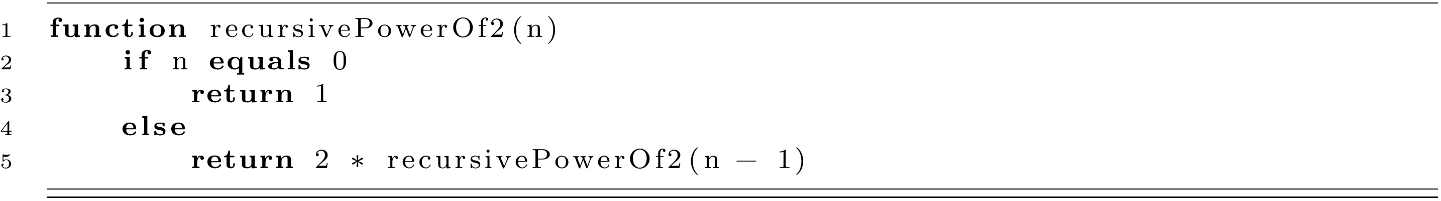
To analyze the complexity of this algorithm, let us examine some example input values. For an n equal to 1, the algorithm begins with recursivePowerOf2(1). This call evaluates 2 * recursivePowerOf2(1). This expression then becomes 2 * 1, which is 2. For an n equal to 3, we have the following sequence:

recursivePowerOf2(3) -> 2 * recursivePowerOf2(2)

-> 2 * 2 * recursivePowerOf2(1)

-> 2 * 2 * 2 * recursivePowerOf2(0)

-> 2 * 2 * 2 * 1

So for an n equal to 3, we have three multiplications. From this expansion of the calls, we can see that this process ultimately resembles the iterative process in terms of the number of steps. We could imagine that for an n equal to 6, recursivePowerOf2(6) would expand into 2 * 2 * 2 * 2 * 2 * 2 * 1 equivalent to the iterative process. From this, we can reason that the time complexity of this recursive algorithm is O(n). This general pattern is sometimes called a linear recursive process.

The time complexity of recursive algorithms can also be calculated using a recurrence relation. Suppose that we let T(n) represent the actual worst-case runtime of a recursive algorithm with respect to the input n. We can then write the time complexity for this algorithm as follows:

This makes sense, as the time complexity is just the cost of one multiplication plus the cost of running the algorithm again with an input of n − 1 (whatever that may be). When n is 0, we must return the value 1. This return action counts as a step in the algorithm.

Now we can use some substitution techniques to solve this recurrence relation:

Here we start to notice a pattern. If we continue this out to T(n − n) = T(0), we can solve the relationship:

We see that T(n) = n + 1, which represents the worst-case time complexity of the algorithm. Therefore, the algorithm’s time complexity is O(n + 1) = O(n).

Next, let us analyze the space complexity. You may try to approach this problem by checking the number of variables used in the recursive procedure that implements this algorithm. Unfortunately, recursion hides some of the memory demands due to the way procedures are implemented with the runtime stack. Though it appears that only one variable is used, every call to the recursive procedure keeps its own separate value for n. This leads to a memory demand that is proportional to the number of calls made to the recursive procedure. This behavior is illustrated in the following figure, which presents a representation of the runtime stack at a point in the execution of the algorithm. Assume that recursivePowerOf2(3) has been called inside main or another procedure to produce a result, and we are examining the stack when the last call to recursivePowerOf2(0) is made during this process.

Figure 2.9

The number of variables needed to calculate recursivePowerOf2(3) is proportional to the size of the input. The figure showing the call stack has a frame for each call starting with 3 and going down to 0. If our input increased, our memory demand would also increase. This observation leads to the conclusion that this algorithm requires O(n) space in the worst case.

Tail-Call Optimization

In considering the two previous algorithms, we can compare them in terms of their time and space scaling behavior. The imperative powerOf2 implementation uses a loop. This algorithm has a time complexity of O(n) and a space complexity of O(1). The recursivePowerOf2 algorithm has a time complexity of O(n), but its space complexity is much worse at O(n). Fortunately, an optimization trick exists that allows recursive algorithms to reduce their space usage. This trick is known as tail-call optimization. If your language or compiler supports tail-call optimization, recursive algorithms can be structured to use the same amount of space as their corresponding iterative implementations. Actually, both algorithms would be considered iterative, as they iteratively update a fixed set of state variables. Let us examine a tail-call optimization example in greater detail.

To fix our recursivePowerOf2 implementation’s space complexity issues, we will first slightly modify our algorithm. We will add a state variable that will hold the running product. This serves the same purpose as the product variable in our iterative loop implementation.

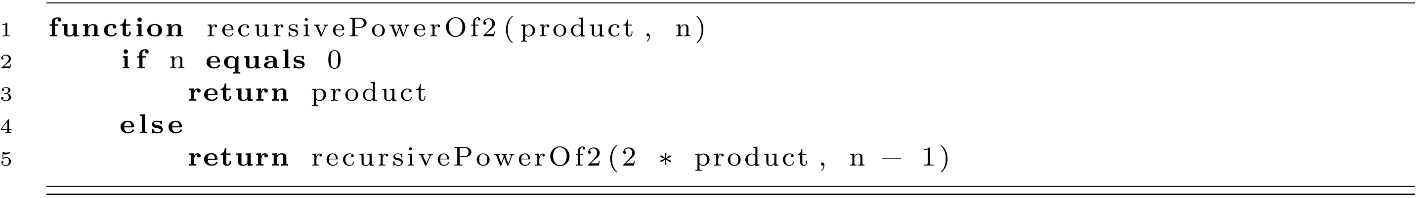
For this algorithm to work correctly, any external call should be made with product set to 1. This ensures that an exponent of n equal to 0 returns 1. This means it would be a good idea to wrap this algorithm in a wrapper function to avoid unnecessary errors when a programmer mistakenly calls the algorithm without product set to 1. This simple wrapper function is presented below:

To understand how tail-call optimization works, let us think about what would happen on the stack when we made a call like recursivePowerOf2(1, 3) using our new algorithm (we will ignore the wrapper for this discussion). The stack without tail-call optimization would look like the following figure:

Figure 2.10

The key observation of tail-call optimization is that when the recursive call is at the tail end of the procedure (in this case, line 5), no information is needed from the current stack frame. This means that the current frame can simply be reused without consuming more memory. The following figure gives an illustration of recursivePowerOf2(1, 3) after the first recursive tail-call in the execution process.

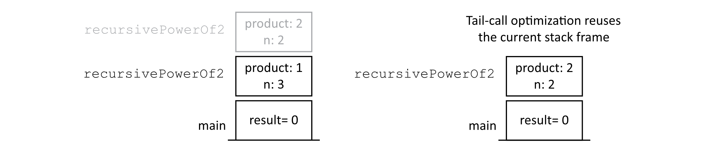
Figure 2.11

Using tail-call optimization, our new recursivePowerOf2 algorithm has the same time complexity O(n) and space complexity O(1) as the loop-based iterative implementation. Keep in mind that tail-call optimization is a feature of either your interpreter or the compiler. You may wish to check if it is supported by your language (https://en.wikipedia.org/wiki/Tail_call#By_language).

Powers of 2 in O(log n) Time

A clever algorithm is presented in Structure and Interpretation of Computer Programs (SICP, Abelson and Sussman, 1996) that calculates powers of any base in O(log n) time. Let us examine this algorithm to help us understand some recursive algorithms that are faster—or rather, scale better—than O(n) time.

We will examine the same problem as above, calculating the nth power of 2. The key idea of this algorithm takes advantage of the fact that 2ⁿ = (2^n/2)² when n is even and 2 * 2ⁿ⁻¹ when n is odd. To implement this algorithm, we must first define two helper functions. One function will square an input number, and the other function will check if a number is even. We will define them here using mod to indicate the remainder after division.

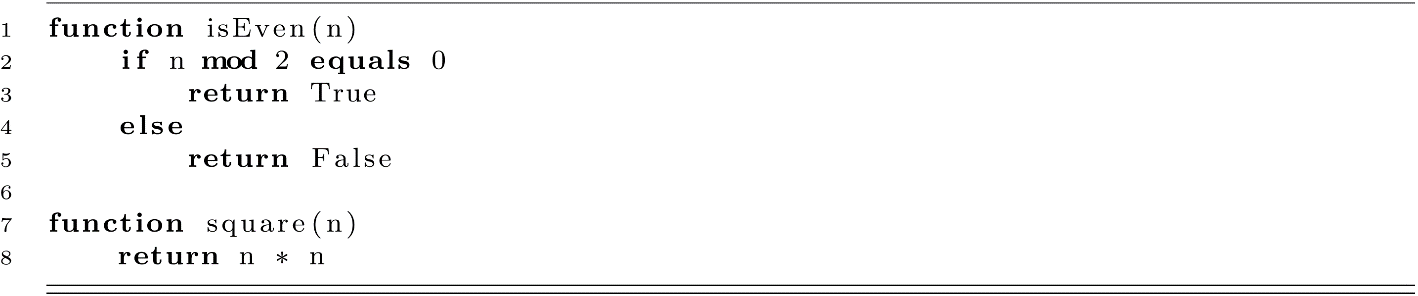
After defining these two functions, we will consider the bases and recursive cases for which we need to account. If n is 0, the algorithm should return 1 according to the mathematical definition of any base value raised to an exponent of 0. This will be one of our cases. Next, if the n is even, we will square the result of a recursive call to the algorithm passing the value of n/2. This code is equivalent to our calculation of (2^n/2)². Lastly, for the odd case, we will calculate 2 times the result of a recursive call that passes the value of n − 1. This code handles the odd case equivalent to 2 * 2ⁿ⁻¹ and sets up the use of our efficient even exponent case. The algorithm is presented below:

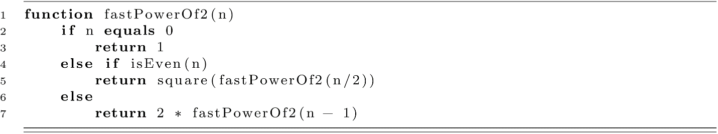
Let us think about the process this algorithm uses to calculate 2⁹. This process starts with a call to fastPowerOf2(9). Since 9 is odd, we would multiply 2 * fastPowerOf2(8). This expression then expands to 2 * square(fastPowerOf2(4)). Let us look at this in more detail.

fastPowerOf2(9)->2 * fastPowerOf2(8)

->2 * square(fastPowerOf2(4))

->2 * square(square(fastPowerOf2(2)))

->2 * square(square(square(fastPowerOf2(1))))

->2 * square(square(square(2 * fastPowerOf2(0))))

->2 * square(square(square(2 * 1)))

->2 * square(square(4))

->2 * square(16)

->2 * 256

->512

It may not be clear that this algorithm is faster than the previous recursivePowerOf2, which was bounded by O(n). Considering the linear calculation of 2⁹ would look like this: 2 * 2 * 2 * 2 * 2 * 2 * 2 * 2 * 2 with 9 multiplications. For this algorithm, we could start thinking about the calculation that is equivalent to 2 * square(square(square(2 * 1))). Our first multiplication is 2 * 1. Next, the square procedure multiplies 2 * 2 to get 4. Then 4 is squared, and then 16 is squared for 2 more multiplications. Finally, we get 2 * 256, giving the solution of 512 after only 5 multiply operations. At least for an n of 9, fastPowerOf2 uses fewer multiply operations. From this, we could imagine that for larger values of n, the fastPowerOf2 algorithm would yield even more savings with fewer total operations compared to the linear algorithm.

Let us now examine the time complexity of fastPowerOf2 using a recurrence relation. The key insight is that roughly every time the recursive algorithm is called, n is cut in half. We could model this as follows: Let us assume that there is a small constant number of operations associated with each call to the recursive procedure. We will represent this as c. Again, we will use the function T(n) to represent the worse-case number of operations for the algorithm. So for this algorithm, we have T(n) = c + T(n/2). Let us write this and the base case as a recurrence relation:

To solve this recurrence problem, we begin by making substitutions and looking for a pattern:

We are beginning to see a pattern, but it may not be perfectly clear. The key is in determining how many of those constant terms there will be once the expression of T(n/x) becomes 1 or 0. Let us rewrite these terms in a different way:

Now we seek a pattern that is a little clearer:

So when will n/2^k be 1?

We can solve for k in the following equation:

Now taking the log₂ of each side gives the following:

Now we can rewrite the original formula:

According to our algorithm, with n equal to 1, we use the odd case giving 2 * fastPowerOf2(0) = 1. So we could reason that T(1) = 2c. Finally, we can remove the recursive terms and with a little rewriting arrive at the time complexity:

Therefore, our asymptotic time complexity is O(log n)

Here we have some constants and lower-order terms that lead us to a time complexity of O(log n). This means that the scaling behavior of fastPowerOf2 is much, much better than our linear version. For reference, suppose n was set to 1,000. A linear algorithm would take around 1,000 operations, whereas an O(log n) algorithm would only take around 20 operations.

As for space complexity, this algorithm does rely on a nested call that needs information from previous executions. This requirement is due to the square function that needs the result of the recursive call to return. This implementation is not tail-recursive. In determining the space complexity, we need to think about how many nested calls need to be made before we reach a base case to signal the end of recursion. For a process like this, all these calls will consume memory by storing data on the runtime stack. As n is divided each time, we will reach a base case after O(log n) recursive calls. This means that in the worst case, the algorithm will have O(log n) stack frames taking up memory. Put simply, its space complexity is O(log n).

References

Abelson, Harold, and Gerald Jay Sussman. Structure and Interpretation of Computer Programs. The MIT Press, 1996.