Introduction

In chapter 4, we explored a very important class of problems: searching. As the number of items increases, Linear Search becomes very costly, as every search costs O(n). Additionally, the real-world time cost of searching increases when the number of searches (also called queries) increases. For this reason, we explored sorting our “keys” (our unique identifiers) and then using Binary Search on data sets that get searched a lot. Binary Search improves our performance to O(log n) for searches. In this chapter, we explore ways to further improve search to approximately O(1) or constant time on average. There are some considerations, but with a good design, searches can be made extremely efficient. The key to this seemingly magic algorithm is the hash function. Let’s explore hashes a bit more in-depth.

Hash Functions

If you have ever eaten breakfast at a diner in the USA, you were probably served some hash browns. These are potatoes that have been very finely chopped up and cooked. In fact, this is where the “hash” of the hash function gets its name. A hash function takes a number, the key, and generates a new number using information in the original key value. So at some level, it takes information stored in the key, chops the bits or digits into parts, then rearranges or combines them to generate a new number. The important part, though, is that the hash function will always generate the same output number given the input key. There are many different types of hash functions. Let’s look at a simple one that hashes the key 137. We will use a small subscript of 2 when indicating binary numbers.

Figure 7.1

We can generate hashes using strings or text as well. We can extract letters from the string, convert them to numbers, and add them together. Here is an example of a different hash function that processes a string:

Figure 7.2

There are many hash functions that can be constructed for keys. For our purposes, we want hash functions that exhibit some special properties. In this chapter, we will be constructing a lookup table using hashes. Suppose we wanted to store student data for 100 students. If our hash function could take the student’s name as the key and generate a unique index for every student, we could store all their data in an array of objects and search using the hash. This would give us constant time, or O(1), lookups for any search! Students could have any name, which would be a vast set of possible keys. The hash function would look at the name and generate a valid array index in the range of 0 to 99.

The hash functions useful in this chapter map keys from a very large domain into a small range represented by the size of the table or array we want to use. Generally, this cannot be done perfectly, and we get some “collisions” where different keys are hashed to the same index. This is one of the main problems we will try to fix in this chapter. So one property of the hash function we want is that it leads to few collisions. Since a perfect hash is difficult to achieve, we may settle for an unbiased one. A hash function is said to be uniform if it hashes keys to indexes with roughly equal probability. This means that if the keys are uniformly distributed, the generated hash values from the keys should also be roughly uniformly distributed. To state that another way, when considered over all k keys, the probability h(k) = a is approximately the same as the probability that h(k) = b. Even with a nice hash function, collisions can still happen. Let’s explore how to tackle these problems.

Hash Tables

Once you have finished reading this chapter, you will understand the idea behind hash tables. A hash table is essentially a lookup table that allows extremely fast search operations. This data structure is also known as a hash map, associative array, or dictionary. Or more accurately, a hash table may be used to implement associative arrays and dictionaries. There may be some dispute on these exact terms, but the general idea is this: we want a data structure that associates a key and some value, and it must efficiently find the value when given the key. It may be helpful to think of a hash table as a generalization of an array where any data type can be used as an index. This is made possible by applying a hash function to the key value.

For this chapter, we will keep things simple and only use integer keys. Nearly all modern programming languages provide a built-in hash function or several hash functions. These language library–provided functions can hash nearly all data types. It is recommended that you use the language-provided hash functions in most cases. These are functions that generally have the nice properties we are looking for, and they usually support all data types as inputs (rather than just integers).

A Hash Table Using Open Addressing

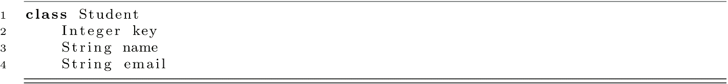
Suppose we want to construct a fast-access database for a list of students. We will use the Student class from chapter 4. We will slightly alter the names though. For this example, we will use the variable name key rather than member_id to simplify the code and make the meaning a bit clearer.

We want our database data structure to be able to support searches using a search operation. Sometimes the term “find” is used rather than “search” for this operation. We will be consistent with chapter 4 and use the term “search” for this operation. As the database will be searched frequently, we want search to be very efficient. We also need some way to add and remove students from the database. This means our data structure should support the add and remove operations.

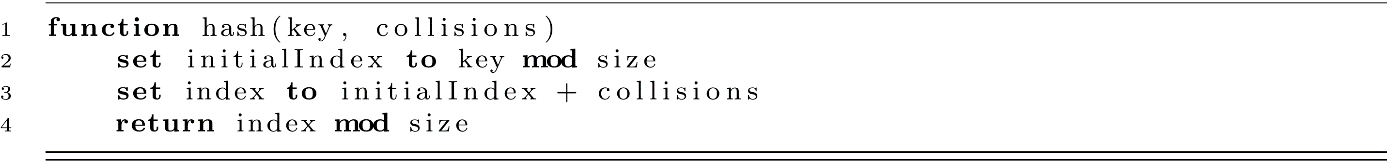
The first strategy we will explore with hash tables is known as open addressing. This means that we will allot some storage space in memory and place new data records into an open position addressed by the hash function. This is usually done using an array. Let the variable size represent the number of positions in the array. With the size of our array known, we can introduce a simple hash function where mod is the modulo or remainder operator.

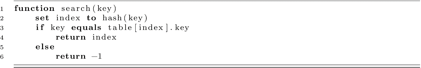
This hash function maps the key to a valid array index. This can be done in constant time, O(1). When searching for a student in our database, we could do something like this:

This would ensure a constant-time search operation. There is a problem, though. Suppose our array had a size of 10. What would happen if we searched for the student with key 18 and another student with key 28? Well, 18 mod 10 is 8, and 28 mod 10 is 8. This simple approach tries to look for the same student in the same array address. This is known as a collision or a hash collision.

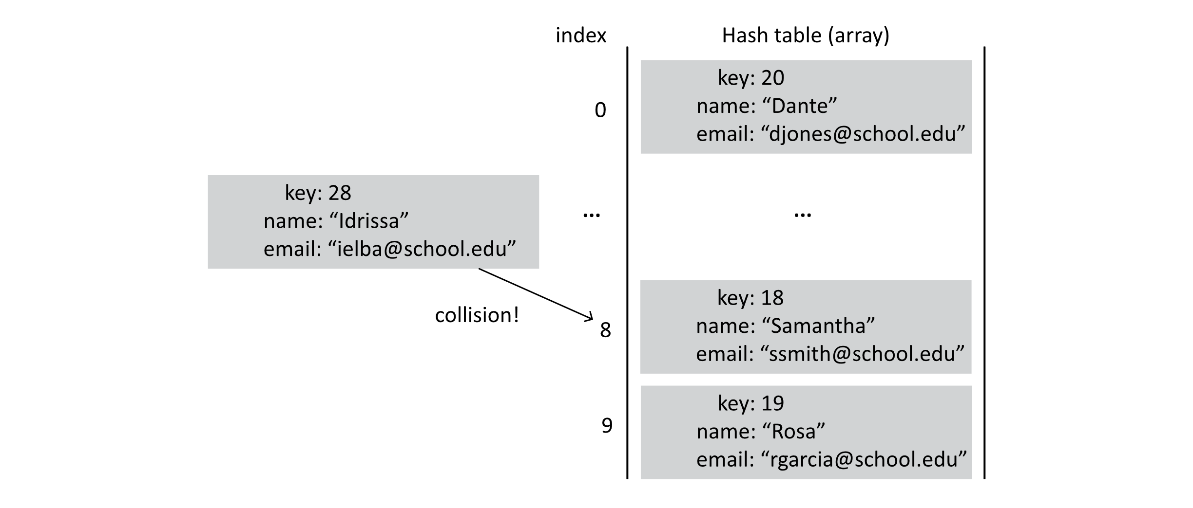
Figure 7.3

We have two options to deal with this problem. First, we could use a different hash function. There may be another way to hash the key to avoid these collisions. Some algorithms can calculate such a function, but they require knowledge of all the keys that will be used. So this is a difficult option most of the time. The second alternative would be to introduce some policy for dealing with these collisions. In this chapter, we will take the second approach and introduce a strategy known as probing. Probing tries to find the correct key by “probing” or checking other positions relative to the initial hashed address that resulted in the collision. Let’s explore this idea with a more detailed example and implementation.

Open Addressing with Linear Probing

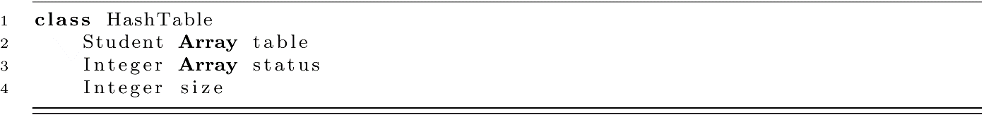
Let us begin by specifying our hash table data structure. This class will need a few class functions that we will specify below, but first let’s give our hash table some data. Our table will need an array of Student records and a size variable.

To add new students to our data structure, we will use an add function. There is a simple implementation for this function without probing. We will consider this approach and then improve on it. Assume that the add function belongs to the HashTable class, meaning that table and size are both accessible without passing them to the function.

Once a student is added, the HashTable could find the student using the search function. We will have our search function return the index of the student in the array or −1 if the student cannot be found.

This approach could work assuming our hash was perfect. This is usually not the case though. We will extend the class to handle collisions. First, let’s explore an example of our probing strategy.

Probing

Suppose we try to insert a student, marked as “A,” into the database and find that the student’s hashed position is already occupied. In this example, student A is hashed to position 2, but we have a collision.

Figure 7.4

With probing, we would try the next position in the probe sequence. The probe sequence specifies which positions to try next. We will use a simple probe sequence known as linear probing. Linear probing will have us just try the next position in the array.

Figure 7.5

This figure shows that first we get a collision when trying to insert student A. Second, we probe the next position in the array and find that it is empty, so student A is inserted into this array slot. If another collision happens on the same hash position, linear probing has us continue to explore further into the array and away from the original hash position.

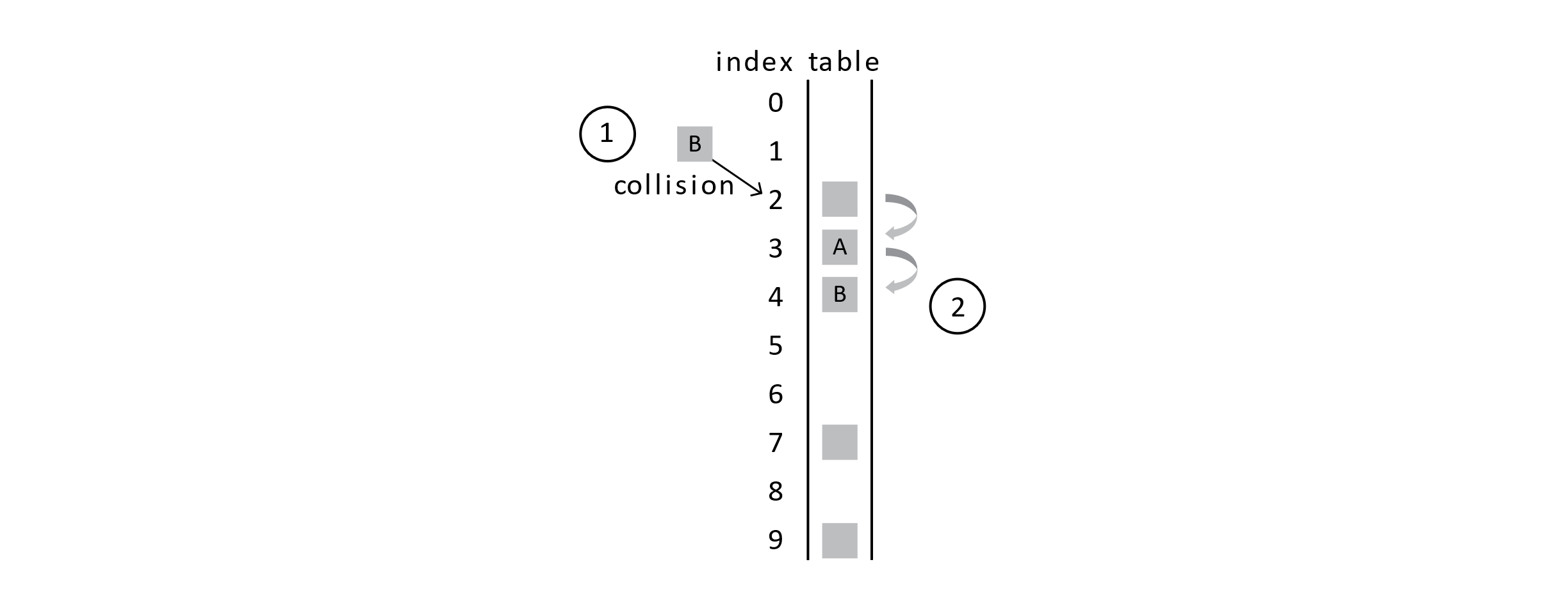
Figure 7.6

This figure shows that another collision will require more probing. You may now be thinking, “This could lead to trouble.” You would be right. Using open addressing with probing means that collisions can start to cause a lot of problems. The frequency of collisions will quickly lead to poor performance. We will revisit this soon when we discuss time complexity. For now, we have a few other problems with this approach.

Add and Search with Probing

Let us tackle a relatively simple problem first. How can we implement our probe sequence? We want our hash function to return the proper hash the first time it is used. If we have a collision, our hash needs to return the original value plus 1. If we have two collisions, we need the original value plus 2, and so on. For this, we will create a new hashing function that takes two input parameters.

With this function, hash(2,2) would give the value 4 as in the previous figure. In that example, when trying to insert student B, we get an initial collision followed by a second collision with student A that was just inserted. Finally, student B is inserted into position 4.

Did you notice the other problem? How will we check to see if the space in the array is occupied? There are a variety of approaches to solving this problem. We will take a simple approach that uses a secondary array of status values. This array will be used to mark which table spaces are occupied and which are available. We will add an integer array called status to our data structure. This approach will simplify the code and prepare our HashTable to support remove (delete) operations. The new HashTable will be defined as follows:

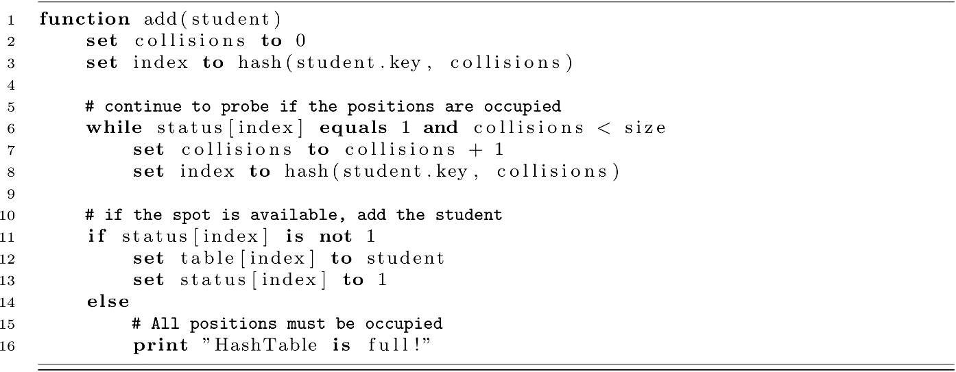
We will assign a status value of 0 to an empty slot and a value of 1 to an occupied slot. Now to check if a space is open and available, the code could just check to see if the status value at that index is 0. If the status is 1, the position is filled, and adding to that location results in a collision. Now let’s use this information to correct our add function for using linear probing. We will assume that all the status values are initialized with 0 when the HashTable is constructed.

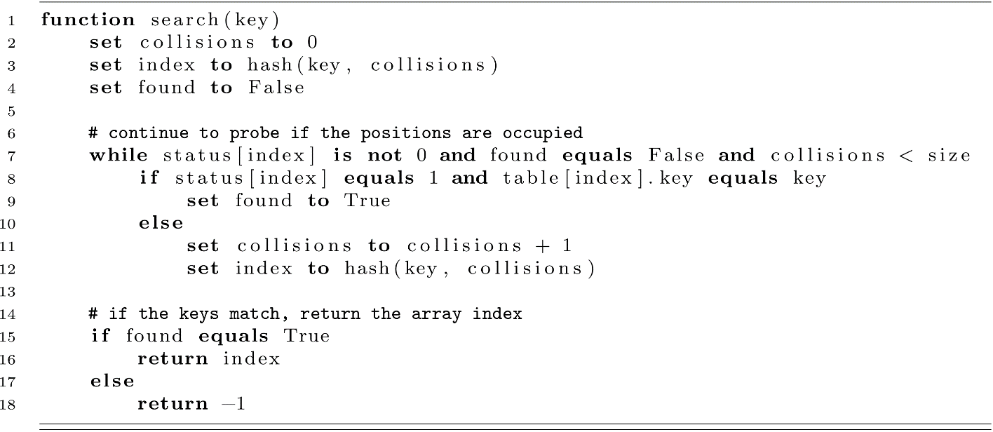
Now that we can add students to the table, let us develop the search function to deal with collisions. The search function will be like add. For this algorithm, status[index] should be 1 inside the while-loop, but we will allow for −1 values a bit later. This is why 0 is not used here.

We need to discuss the last operation now: remove. The remove operation may also be called delete in some contexts. The meaning is the same though. We want a way to remove students from the database. Let’s think about what happens when a student is removed from the database. Think back to the collision example where student B is inserted into the database. What would happen if A was removed and then we searched for B?

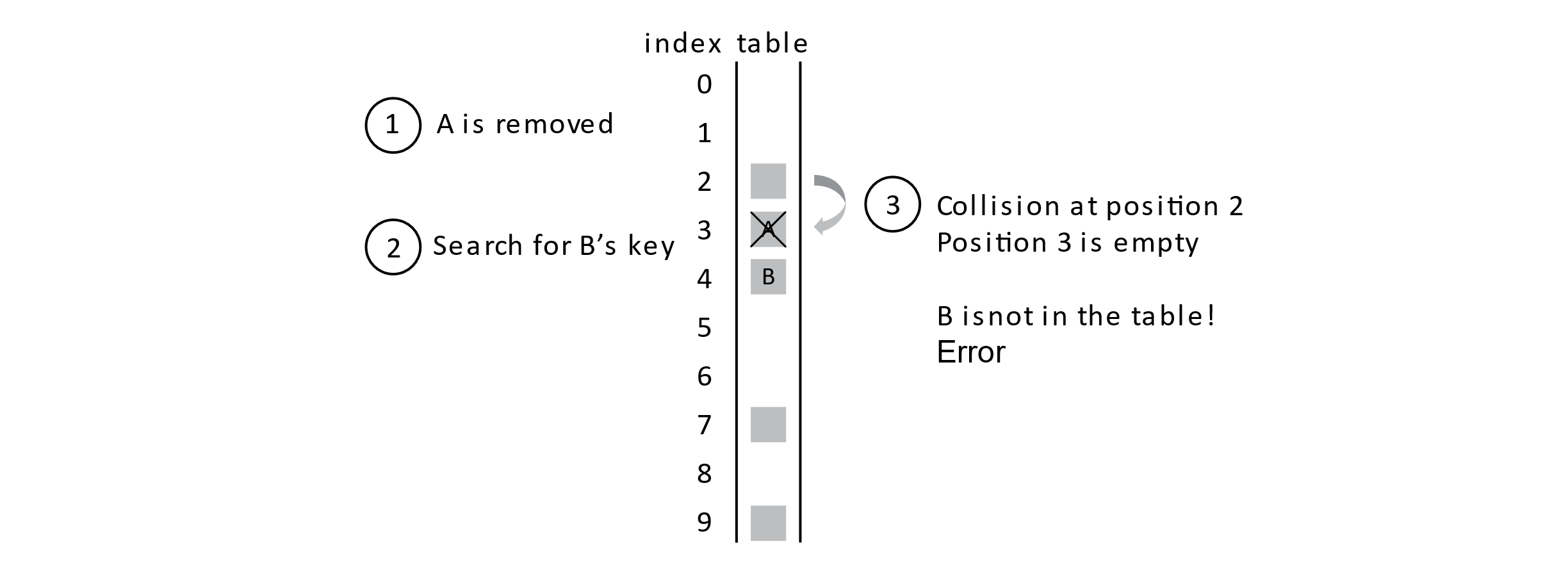
Figure 7.7

If we just marked a position as open after a remove operation, we would get an error like the one illustrated above. With this sequence of steps, it seems like B is not in the table because we found an open position as we searched for it. We need to deal with this problem. Luckily, we have laid the foundation for a simple solution. Rather than marking a deleted slot as open, we will give it a deleted status code. In our status array, any value of −1 will indicate that a student was deleted from the table. This will solve the problem above by allowing searches to proceed past these deleted positions in the probe sequence.

The following function can be used to implement the remove function. This approach relies on our search function that returns the correct index. Notice how the status array is updated.

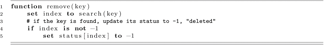
Depending on your implementation, you may also want to free the memory at table[index] at line 5. We are assuming that student records are stored directly in the array and will be overwritten on the next add operation for that position. If references are used, freeing the data may need to be explicit.

Take a careful look back at the search function to convince yourself that this is correct. When the status is −1, the search function should proceed through past collisions to work correctly. We now have a correct implementation of a hash table. There are some serious drawbacks though. Let us now discuss performance concerns with our hash table.

Complexity and Performance

We saw that adding more students to the hash table can lead to collisions. When we have collisions, the probing sequence places the colliding student near the original student record. Think about the situation below that builds off one of our previous examples:

Figure 7.8

Suppose that we try to add student C to the table and C’s key hashes to the index 3. No other student’s key hashes to position 3, but we still get 2 collisions. This clump of records is known as a cluster. You can see that a few collisions lead to more collisions and the clusters start to grow and grow. In this example, collisions now result if we get keys that hash to any index between 2 and 5.

What does this mean? Well, if the table is mostly empty and our hash function does a decent job of avoiding collisions, then add and search should both be very efficient. We may have a few collisions, but our probe sequences would be short and on the order of a constant number of operations. As the table fills up, we get some collisions and some clusters. Then with clustering, we get more collisions and more clustering as a result. Now our searches are taking many more operations, and they may approach O(n) especially when the table is full and our search key is not actually in the database. We will explore this in a bit more detail.

A load factor is introduced to quantify how full or empty the table is. This is usually denoted as α or the Greek lowercase alpha. We will just use an uppercase L. The load factor can be defined as simply the ratio of added elements to the total capacity. In our table, the capacity is represented by the size variable. Let n be the number of elements to be added to the database. Then the overall load factor for the hash table would be L = n / size. For our table, L must be less than 1, as we can only store as many students as we have space in the array.

How does this relate to runtime complexity? Well, in the strict sense, the worst-case performance for searches would be O(n). This is represented by the fact that when the table is full, we must check nearly all positions in the table. On the other hand, our analysis of Quick Sort showed that the expected worst-case performance can mean we get a very efficient and highly useful algorithm even if some cases may be problematic. This is the case with hash tables. Our main interest is in the average case performance and understanding how to avoid the worst-case situation. This is where the load factor comes into play. Donald Knuth is credited with calculating the average number of probes needed for linear probing in both a successful search and the more expensive unsuccessful search. Here, a successful search means that the item is found in the table. An unsuccessful search means the item was searched for but not found to be in the table. These search cost values depend on the L value. This makes sense, as a mostly empty table will be easy to insert into and yield few collisions.

The expected number of probes for a successful search with linear probing is as follows:

For unsuccessful searches, the number of probes is larger:

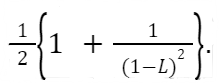
Let’s put these values in context. Suppose our table size is 50 and there are 10 student records inserted into the table giving a load factor of 10/50 = 0.2. This means on average a successful search needs 1.125 probes. If the table instead contains 45 students, we can expect an average of 5.5 probes with an L of 45/50 = 0.9. This is the average. Some may take longer. The unsuccessful search yields even worse results. With an L of 10/50 = 0.2, an unsuccessful search would yield an average of 1.28 probes. With a table of lead L = 45/50 = 0.9, the average number of probes would be 50.5. This is close to the worst-case O(n) performance.

We can see that the average complexity is heavily influenced by the load factor L. This is true of all open addressing hash table methods. For this reason, many hash table data structures will detect that the load is high and then dynamically reallocate a larger array for the data. This increases capacity and reduces the load factor. This approach is also helpful when the table accumulates a lot of deleted entries. We will revisit this idea later in the chapter. Although linear probing has some poor performance at high loads, the nature of checking local positions has some advantages with processor caches. This is another important idea that makes linear probing very efficient in practice.

The space complexity of a hash table should be clear. We need enough space to store the elements; therefore, the space complexity is O(n). This is true of all the open addressing methods.

Other Probing Strategies

One major problem with linear probing is that as collisions occur, clusters begin to grow and grow. This blocks other hash positions and leads to more collisions and therefore more clustering. One strategy to reduce the cluster growth is to use a different probing sequence. In this section, we will look at two popular alternatives to linear probing. These are the methods of quadratic probing and double hashing. Thanks to the design of our HashTable in the previous section, we can simply define new hash functions. This modular design means that changing the functionality of the data structure can be done by changing a single function. This kind of design is sometimes difficult to achieve, but it can greatly reduce repeated code.

Quadratic Probing

One alternative to linear probing is quadratic probing. This approach generates a probe sequence that increases by the square of the number of collisions. One simple form of quadratic probing could be implemented as follows:

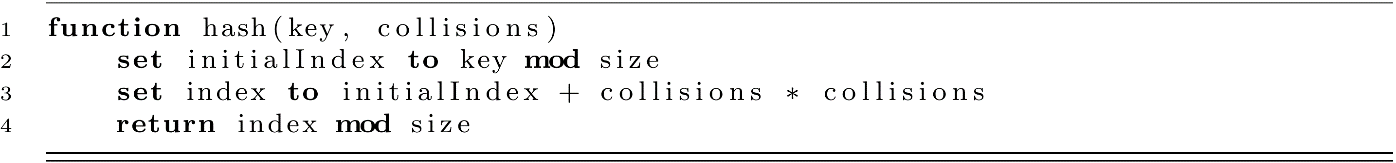
The following illustration shows how this might improve on the problem of clustering we saw in the section on linear probing:

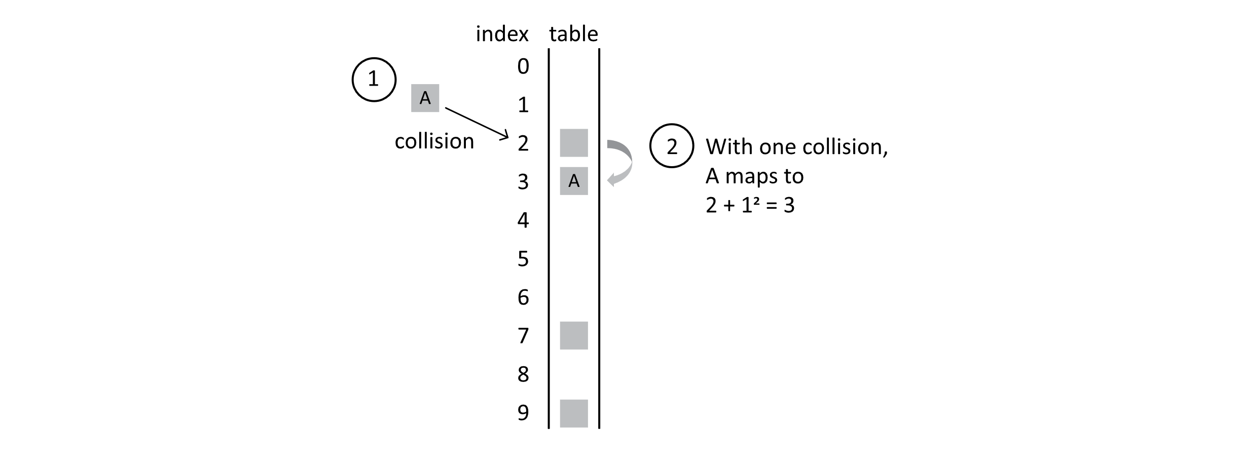
Figure 7.9

With one collision, student A still maps to position 3 because 2 + 1² = 3. When B is mapped though, it results in 2 collisions. Ultimately, it lands in position 6 because 2 + 2² = 6, as the following figure shows:

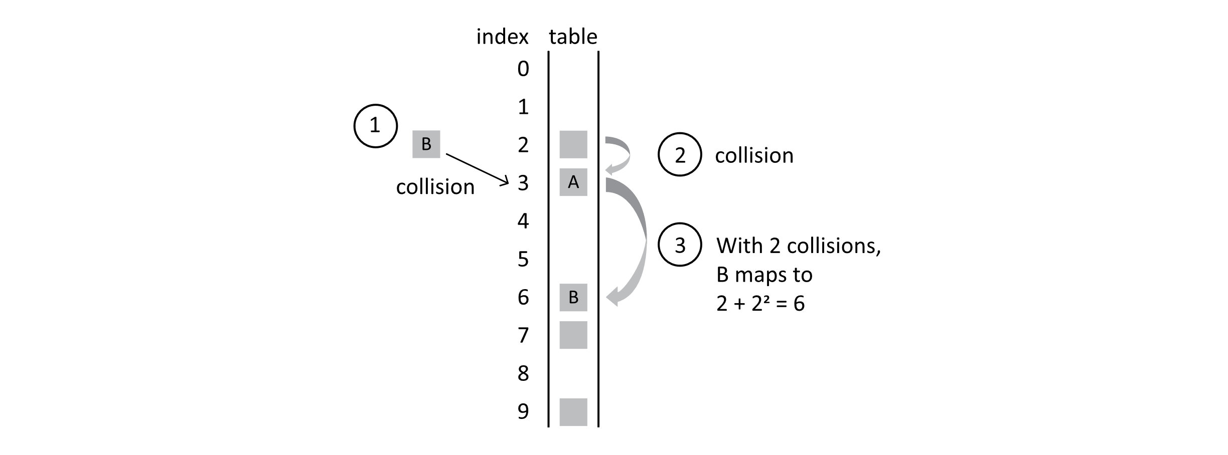
Figure 7.10

When student C is added, it will land in position 4, as 3 + 1² = 4. The following figure shows this situation:

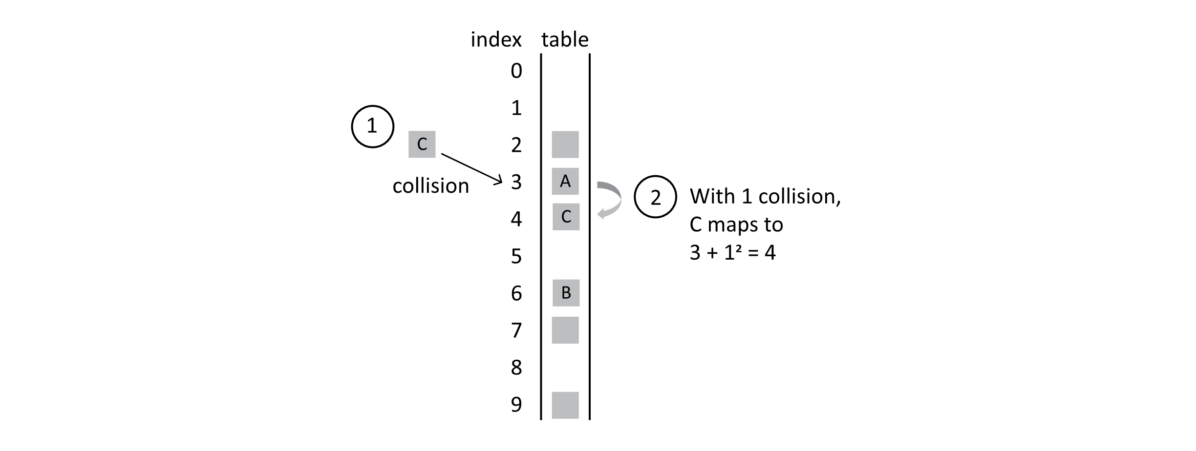
Figure 7.11

Now instead of one large primary cluster, we have two somewhat smaller clusters. While quadratic probing reduces the problems associated with primary clustering, it leads to secondary clustering.

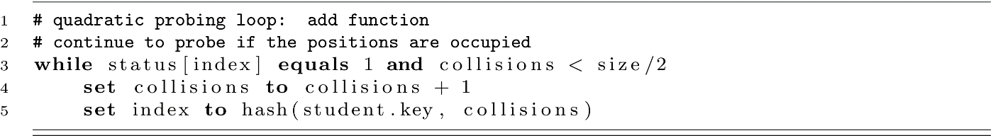
One other problem with quadratic probing comes from the probe sequence. Using the approach we showed where the hash is calculated using a formula like h(k) + c², we will only use about size/2 possible indexes. Look at the following sequence: 1, 4, 9, 16, 25, 36, 49, 64, 81, 100, 121, 144. Now think about taking these values after applying mod 10. We get 1, 4, 9, 6, 5, 6, 9, 4, 1, 0, 1, 4. These give only 6 unique values. The same behavior is seen for any mod value or table size. For this reason, quadratic probing usually terminates once the number of collisions is half of the table size. We can make this modification to our algorithm by modifying the probing loop in the add and search functions.

For the add function, we would use

For the search function, we would use

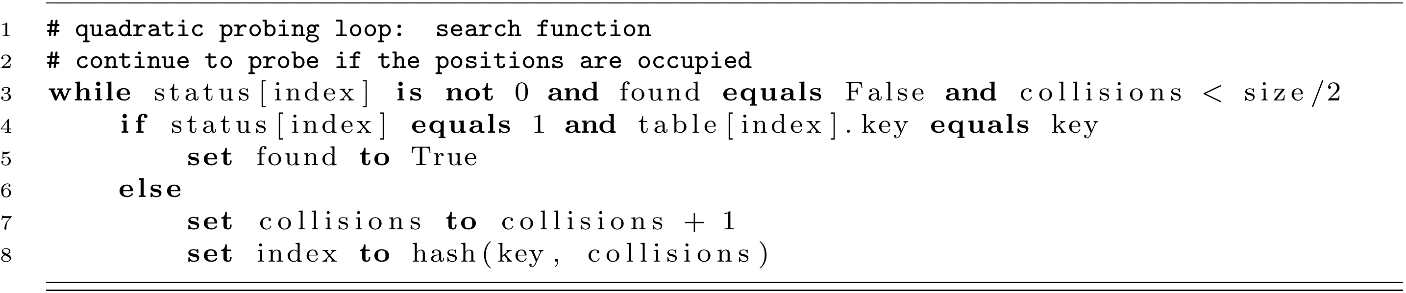
When adding, it is assumed that encountering size/2 collisions means that the table is full. It is possible that this is incorrect. There may be open positions available even after quadratic probing has failed. If attempting to add fails, it is a good indicator that the load factor has become too high anyway, and the table needs to be expanded and rebuilt.

Double Hashing

In this section, we will look at an implementation of a hashing collision strategy that approaches the ideal strategy for an open addressed hash table. We will also discuss how to choose a good table size such that our hash functions perform better when our keys do not follow a random uniform distribution.

Choosing a Table Size

So far, we have chosen a table size of 10 in our examples. This has made it easy to think about what hash value is generated from a base-10 numerical key. This would be fine assuming our key distribution was truly uniform in the key domain. In practice, keys can have some properties that result in biases and ultimately nonuniform distributions. Take, for example, the use of a memory address as a key. On many computer systems, memory addresses are multiples of 4. As another example, in English, the letter “e” is far more common than other letters. This might result in keys generated from ASCII text having a nonuniform distribution.

Let’s look at an example of when this can become a problem. Suppose we have a table of size 12 and our keys are all multiples of 4. This would result in all keys being initially hashed to only the indexes 0, 4, or 8. For both linear probing and quadratic probing, any key with the initial hash value will give the same probing sequence. So this example gives an especially bad situation resulting in poor performance under both linear probing and quadratic probing. Now suppose that we used a prime number rather than 12, such as 13. The table below gives a sequence of multiples of 4 and the resulting mod values when divided by 12 and 13.

Figure 7.12

It is easy to see that using 13 performs much better than 12. In general, it is favored to use a table size that is a prime value. The approach of using a prime number in hash-based indexing is credited to Arnold Dumey in a 1956 work. This helps with nonuniform key distributions.

Implementing Double Hashing

As the name implies, double hashing uses two hash functions rather than one. Let’s look at the specific problem this addresses. Suppose we are using the good practice of having size be a prime number. This still cannot overcome the problem in probing methods of having the same initial hash index. Consider the following situation. Suppose k₁ is 13 and k₂ is 26. Both keys will generate a hashed value of 0 using mod 13. The probing sequence for k₁ in linear probing is this:

Quadratic probing has the same problem:

Let’s walk through the quadratic probing sequence a little more carefully to make it clear. Recall that

using quadratic probing. The following table gives the probe sequence for k₁ = 13 and k₂ = 26 using quadratic probing:

Figure 7.13

The probe sequence is identical given the same initial hash. To solve this problem, double hashing was introduced. The idea is simple. A second hash function is introduced, and the probe sequence is generated by multiplying the number of collisions by a second hash function. How should we choose this second hash function? Well, it turns out that choosing a second prime number smaller than size works well in practice.

Let’s create two hash functions h₁(k) and h₂(k). Now let p₁ be a prime number that is equal to size. Let p₂ be a prime number such that p₂ < p₁. We can now define our functions and the final double hash function:

The final function to generate the probe sequence is here:

Let’s let p₁ = 13 = size and p₂ = 11 for our example. How would this change the probe sequence for our keys 13 and 26? In this case h₁(13) = h₁(26) = 0, but h₂(13) = 2, h₂(26) = 4.

Consider the following table:

Figure 7.14

Now that we understand double hashing, let’s start to explore one implementation in code. We will create two hash functions as follows:

The second hash function will use a variable called prime, which has a value that is a prime number smaller than size.

Finally, our hash function with a collisions parameter is developed below:

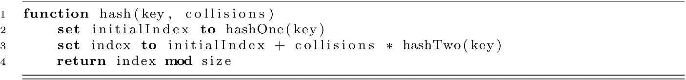
As before, these can be easily added to our HashTable data structure without changing much of the code. We would simply add the hashOne and hashTwo functions and replace the two-parameter hash function.

Complexity of Open Addressing Methods

Open addressing strategies for implementing hash tables that use probing all have some features in common. Generally speaking, they all require O(n) space to store the data entries. In the worst case, search-time cost could be as bad as O(n), where the data structure checks every entry for the correct key. This is not the full story though.

As we discussed before with linear probing, when a table is mostly empty, adding data or searching will be fast. First, check the position in O(1) with the hash. Next, if the key is not found and the table is mostly empty, we will check a small constant number of probes. Search and insert would be O(1), but only if it’s mostly empty. The next question that comes to mind is “What does ‘mostly empty’ mean?” Well, we used a special value to quantify the “fullness” level of the table. We called this the load factor, which we represented with L.

Let’s explore L and how it is used to reason about the average runtime complexity of open addressing hash tables. To better understand this idea, we will use an ideal model of open addressing with probing methods. This is known as uniform hashing, which was discussed a bit before. Remember the problems of linear probing and quadratic probing. If any value gives the same initial hash, they end up with the same probe sequence. This leads to clustering and degrading performance. Double hashing is a close approximation to uniform hashing. Let’s consider double hashing with two distinct keys, k₁ and k_2. We saw that when h₁(k₁) = h₁(k₂), we can still get a different probe sequence if h₂(k₁) ≠ h₂(k₂). An ideal scenario would be that every unique key generates a unique but uniform random sequence of probe indexes. This is known as uniform hashing. Under this model, thinking about the average number of probes in a search is a little easier. Let’s think this through.

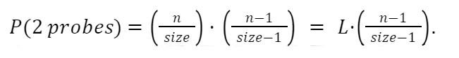
Remember that the load on the table is the ratio of filled to the total number of available positions in the table. If n elements have been inserted into the table, the load is L = n / size. Let’s consider the case of an unsuccessful search. How many probes would we expect to make given that the load is L? We will make at least one check, but next, the probability that we would probe again would be L. Why? Well, if we found one of the (size − n) open positions, the search would have ended without probing. So the probability of one unsuccessful probe is L. What about the probability of two unsuccessful probes? The search would have failed in the first probe with probability L, and then it would fail again in trying to find one of the (n − 1) occupied positions among the (size − 1) remaining available positions. This leads to a probability of

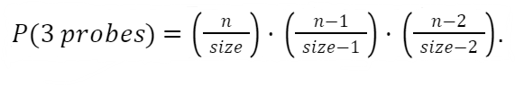
Things would progress from there. For 3 probes, we get the following:

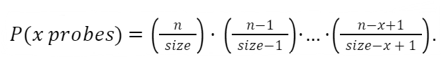
On and on it goes. We extrapolate out to x probes:

This sequence would be smaller than assuming a probability of L for every missed probe. We could express this relationship with the following equation:

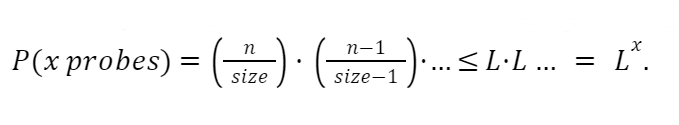
This gives us the probability of having multiple failed probes. We now want to think about the expected number of probes. One failed probe has the probability of L, and having more failed probes is less likely. To calculate the expected number of probes, we need to add the probabilities of all numbers of probes. So the P(1 probe) + P(2 probes)…on to infinity. You can think of this as a weighted average of all possible numbers of probes. A more likely number of probes contributes more to the weighted average. It turns out that we can calculate a value for this infinite series. The sum will converge to a specific value. We arrive at the following formula using the geometric series rule to give a bound for the number of probes in an unsuccessful search:

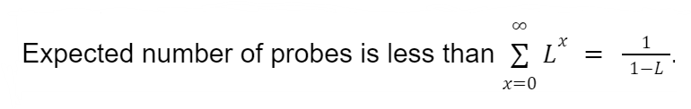
This equation bounds the expected number of probes or comparisons in an unsuccessful search. If 1/(1−L) is constant, then searches have an average case runtime complexity of O(1). We saw this in our analysis of linear probing where the performance was even worse than for the ideal uniform hashing.

For one final piece of analysis, look at the plot of 1/(1−L) between 0 and 1. This demonstrates just how critical the load factor can be in determining the expected complexity of hashing. This shows that as the load gets very high, the cost rapidly increases.

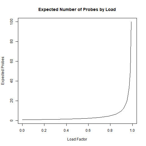Figure 7.15

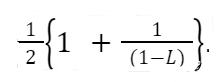
For completeness, we will present the much better performance of a successful search under uniform hashing:

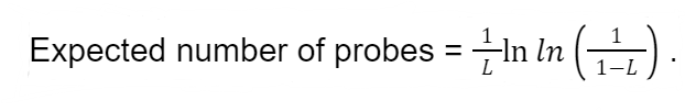
Successful searches scale much better than unsuccessful ones, but they will still approach O(n) as the load gets high.

Chaining

An alternative strategy to open addressing is known as chaining or separate chaining. This strategy uses separate linked lists to handle collisions. The nodes in the linked list are said to be “chained” together like links on a chain. Our records are then organized by keeping them on “separate chains.” This is the metaphor that gives the data structure its name. Rather than worrying about probing sequences, chaining will just keep a list of all records that collided at a hash index.

This approach is interesting because it represents an extremely powerful concept in data structures and algorithms, composition. Composition allows data structures to be combined in multiple powerful ways. How does it work? Well, data structures hold data, right? What if that “data” was another data structure? The specific composition used by separate chaining is an array of linked lists. To better understand this concept, we will visualize it and work through an example. The following image shows a chaining-based hash table after 3 add operations. No collisions have occurred yet:

Figure 7.16

The beauty of separate chaining is that both adding and removing records in the table are made extremely easy. The complexity of the add and remove operations is delegated to the linked list. Let’s assume the linked list supports add and remove by key operations on the list. The following functions give example implementations of add and remove for separate chaining. We will use the same Student class and the simple hash function that returns the key mod size.

The add function is below. Keep in mind that table[index] here is a linked list object:

Here is the remove function that, again, relies on the linked list implementation of remove:

When a Student record needs to be added to the table, whether a collision occurs or not, the Student is simply added to the linked list. See the diagram below:

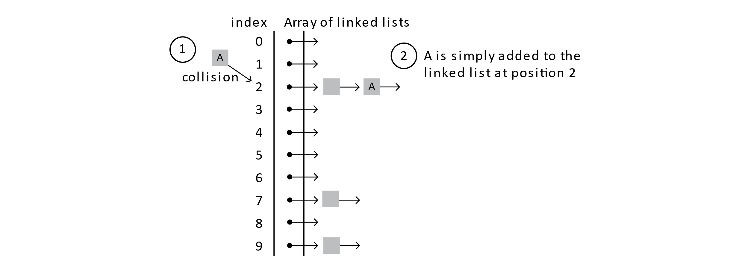Figure 7.17

When considering the implementation, collisions are not explicitly considered. The hash index is calculated, and student A is inserted by asking the link list to insert it. Let’s follow a few more add operations.

Suppose a student, B, is added with a hash index of 2.

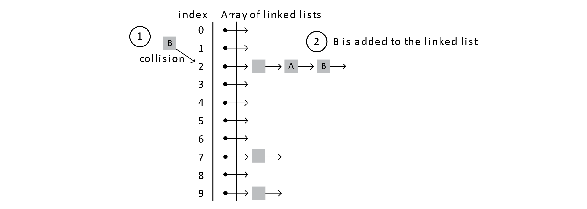
Figure 7.18

Now if C is added with a hash index of 3, it would be placed in the empty list at position 3 in the array.

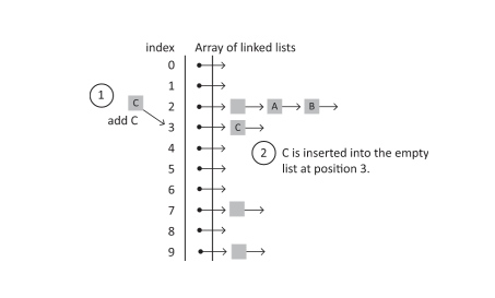
Figure 7.19

Here, the general idea of separate chaining is clear. Maybe it is also clear just how this could go wrong. In the case of search operations, finding the student with a given key would require searching for every student in the corresponding linked list. As you know from chapter 4, this is called Linear Search, and it requires O(n) operations, where n is the number of items in the list. For the separate chaining hash table, the length of any of those individual lists is hoped to be a small fraction of the total number of elements, n. If collisions are very common, then the size of an individual linked list in the data structure would get long and approach n in length. If this can be avoided and every list stays short, then searches on average take a constant number of operations leading to add, remove, and search operations that require O(1) operations on average. In the next section, we will expand on our implementation of a separate chaining hash table.

Separate Chaining Implementation

For our implementation of a separate chaining hash table, we will take an object-oriented approach. Let us assume that our data are the Student class defined before. Next, we will define a few classes that will help us create our hash table.

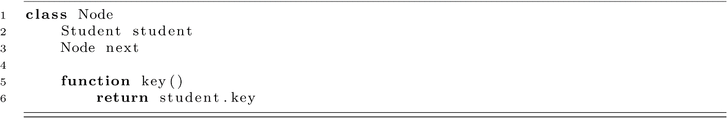
We will begin by defining our linked list. You may want to review chapter 4 before proceeding to better understand linked lists. We will first define our Node class and add a function to return the key associated with the student held at the node. The node class holds the connections in our list and acts as a container for the data we want to hold, the student data. In some languages, the next variable needs to be explicitly declared as a reference or pointer to the next Node.

We will now define the data associated with our LinkedList class. The functions are a little more complex and will be covered next.

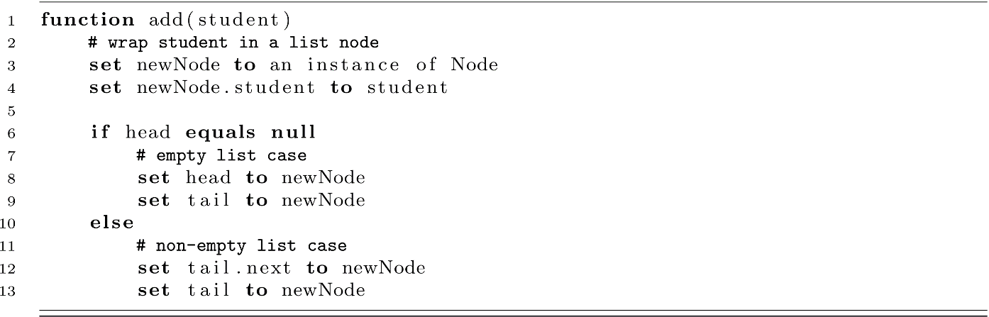
Our list will just keep track of references to the head and tail Nodes in the list. To start thinking about using this list, let’s cover the add function for our LinkedList. We will add new students to the end of our list in constant time using the tail reference. We need to handle two cases for add. First, adding to an empty list means we need to set our head and tail variables correctly. All other cases will simply append to the tail and update the tail reference.

Searching in the list will use Linear Search. Using the currentNode reference, we check every node for the key we are looking for. This will give us either the correct node or a null reference (reaching the end of the list without finding it).

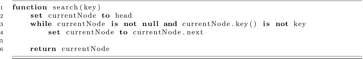
You may notice that we return currentNode regardless of whether the key matches or not. What we really want is either a Student object or nothing. We sidestepped this problem with open addressing by returning −1 when the search failed or the index of the student record when it was found. This means upstream code needs to check for the −1 before doing something with the result. In a similar way here, we send the problem upstream. Users of the code will need to check if the returned node reference is null. There are more elegant ways to solve this problem, but they are outside of the scope of the textbook. Visit the Wikipedia article on the Option Type for some background. For now, we will ask the user of the class to check the returned Node for the Student data.

To finish our LinkedList implementation for chaining, we will define our remove function. As remove makes modifications to our list structure, we will take special care to consider the different cases that change the head and tail members of the list. We will also use the convention of returning the removed node. This will allow the user of the code to optionally free its memory.

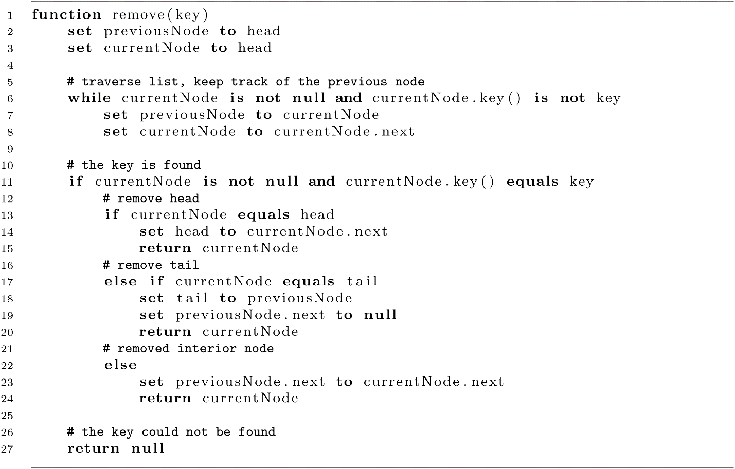
Now we will define our hash table with separate chaining. In the next code piece, we will define the data of our HashTable implemented with separate chaining. The HashTable’s main piece of data is the composed array of LinkedLists. Also, the simple hash function is defined (key mod size).

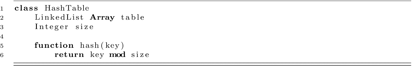
Here the simplicity of the implementation shines. The essential operations of the HashTable are delegated to LinkedList, and we get a robust data structure without a ton of programming effort! The functions for the add, search, and remove operations are presented below for our chaining-based HashTable:

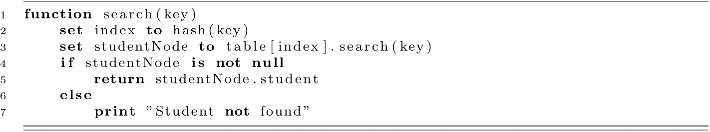
One version of remove is provided below:

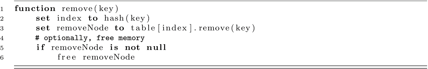
Some implementations of remove may expect a node reference to be given. If this is the case, remove could be implemented in constant time assuming the list is doubly linked. This would allow the node to be removed by immediately accessing the next and previous nodes. We have taken the approach of using a singly linked list and essentially duplicating the search functionality inside the LinkedList’s remove function.

Not bad for less than 30 lines of code! Of course, there is more code in each of the components. This highlights the benefit of composition. Composing data structures opens a new world of interesting and useful data structure combinations.

Separate Chaining Complexity

Like with open addressing methods, the worst-case performance of search (and our remove function) is O(n). Probing would eventually consider nearly all records in our HashTable. This makes the O(n) complexity clear. Thinking about the worst-case performance for chaining may be a little different. What would happen if all our records were hashed to the same list? Suppose we inserted n Students into our table and that they all shared the same hash index. This means all Students would be inserted into the same LinkedList. Now the complexity of these operations would all require examining nearly all student records. The complexity of these operations in the HashTable would match the complexity of the LinkedList, O(n).

Now we will consider the average or expected runtime complexity. With the assumption that our keys are hashed into indexes following a simple uniform distribution, the hash function should, on average, “evenly” distribute the records along all the lists in our array. Here “evenly” means approximately evenly and not deviating too far from an even split.

Let’s put this in more concrete terms. We will assume that the array for our table has size positions, and we are trying to insert n elements into the table. We will use the same load factor L to represent the load of our table, L = n / size. One difference from our open addressing methods is that now our L variable could be greater than 1. Using linked lists means that we can store more records in all of the lists than we have positions in our array of lists. When n Student records have been added to our chaining-based HashTable, they should be approximately evenly distributed between all the size lists in our array. This means that the n records are evenly split between size positions. On average, each list contains approximately L = n / size nodes. Searching those lists would require O(L) operations. The expected runtime cost for an unsuccessful search using chaining is often represented as O(1 + L). Several textbooks report the complexity this way to highlight the fact that when L is small (less than 1) the cost of computing the initial hash dominates the 1 part of the O(1 + L). If L is large, then it could dominate the complexity analysis. For example, using an array of size 1 would lead to L = n / 1 = n. So we get O(1 + L) = O(1 + n) = O(n). In practice, the value of L can be kept low at a small constant. This makes the average runtime of search O(1 + L) = O(1 + c) for some small constant c. This gives us our average runtime of O(1) for search, just as we wanted!

For the add operation, using the tail reference to insert records into the individual lists gives O(1) time cost. This means adding is efficient. Some textbooks report the complexity of remove or delete to be O(1) using a doubly linked list. If the Node’s reference is passed to the remove function using this implementation, this would give us an O(1) remove operation. This assumes one thing though. You need to get the Node from somewhere. Where might we get this Node? Well, chances are that we get it from a search operation. This would mean that to effectively remove a student by its key requires O(1 + L) + O(1) operations. This matches the performance of our implementation that we provided in the code above.

The space complexity for separate chaining should be easy to understand. For the number of records we need to store, we will need that much space. We would also need some extra memory for references or pointer variables stored in the nodes of the LinkedLists. These “linking” variables increase overall memory consumption. Depending on the implementation, each node may need 1 or 2 link pointers. This memory would only increase the memory cost by a constant factor. The space required to store the elements of a separate chaining HashTable is O(n).

Design Trade-Offs for Hash Tables

So what’s the catch? Hash tables are an amazing data structure that has attracted interest from computer scientists for decades. These hashing-based methods have given a lot of benefits to the field of computer science, from variable lookups in interpreters and compilers to fast implementations of sets, to name a few uses. With hash tables, we have smashed the already great search performance of Binary Search at O(log n) down to the excellent average case performance of O(1). Does it sound too good to be true? Well, as always, the answer is “It depends.” Learning to consider the performance trade-offs of different data structures and algorithms is an essential skill for professional programmers. Let’s consider what we are giving up in getting these performance gains.

The great performance scaling behavior of search is only in the average case. In practice, this represents most of the operations of the hash tables, but the possibility for extremely poor performance exists. While searching on average takes O(1), the worst-case time complexity is O(n) for all the methods we discussed. With open addressing methods, we try to avoid O(n) performance by being careful about our load factor L. This means that if L gets too large, we need to remove all our records and re-add them into a new larger array. This leads to another problem, wasted space. To keep our L at a nice value of, say, 0.75, that means that 25% of our array space goes unused. This may not be a big problem, but that depends on your application and system constraints. On your laptop, a few missing megabytes may go unnoticed. On a satellite or embedded device, lost memory may mean that your costs go through the roof. Chaining-based hash tables do not suffer from wasted memory, but as their load factor gets large, average search performance can suffer also. Again, a common practice is to remove and re-add the table records to a larger array once the load crosses a threshold. It should be noted again though that separate chaining already requires a substantial amount of extra memory to support linking references. In some ways, these memory concerns with hash tables are an example of the speed-memory trade-off, a classic concept in computer science. You will often find that in many cases you can trade time for space and space for time. In the case of hash tables, we sacrifice a little extra space to speed up our searches.

Another trade-off we are making may not be obvious. Hash tables guarantee only that searches will be efficient. If the order of the keys is important, we must look to another data structure. This means that finding the record with key 15 tells us nothing about the location of records with key 14 or 16. Let’s look at an example to better understand this trade-off in which querying a range might be a problem for hash tables compared to a Binary Search.

Suppose we gave every student a numerical identifier when they enrolled in school. The first student got the number 1, the second student got the number 2, and so on. We could get every student that enrolled in a specific time period by selecting a range. Suppose we used chaining to store our 2,000 students using the identifier as the key. Our 2,000 students would be stored in an array of lists, and the array’s size is 600. This means that on average each list contains between 3 and 4 nodes (3.3333…). Now we need to select 20 students that were enrolled at the same time. We need all the records for students whose keys are between 126 to 145 (inclusive). For a hash table, we would first search for key 126, add it to the list, then 127, then 128, and so on. Each search takes about three operations, so we get approximately 3.3333 * 20 = 66.6666 operations. What would this look like for a Binary Search? In Binary Search, the array of records is already sorted. This means that once we find the record with key 126, the record with key 127 is right next to it. The cost here would be log₂(2000) + 20. This supposes that we use one Binary Search and 20 operations to add the records to our return list. This gives us approximately log₂(2000) + 20 = 10.9657 + 20 = 30.9657. That is better than double our hash table implementation. However, we also see that individual searches using the hash table are over 3 times as fast as the Binary Search (10.6657 / 3.333 = 3.2897).

References

Cormen, Thomas H., Charles E. Leiserson, Ronald L. Rivest, and Clifford Stein. Introduction to Algorithms, 2nd ed. Cambridge, MA: The MIT Press, 2001.
Dumey, Arnold I. “Indexing for Rapid Random Access Memory Systems,” Computers and Automation 5, no. 12 (1956): 6–9.
Flajolet, P., P. Poblete, and A. Viola. “On the Analysis of Linear Probing Hashing,” Algorithmica 22, no. 4 (1998): 490–515.
Knuth, Donald E. “Notes on ‘Open’ Addressing.” 1963. https://jeffe.cs.illinois.edu/teaching/datastructures/2011/notes/knuth-OALP.pdf.
Malik, D. S. Data Structures Using C++. Cengage Learning, 2009.