
5 Linked Lists
Learning Objectives
After reading this chapter you will…
- begin to understand how differences in data structures result in trade-offs and help when choosing which to apply in a real-world scenario.
- begin to use links or references to build more complex data structures.
- grasp the power and limitations of common arrays.
Introduction
You have a case of cola you wish to add to your refrigerator. Your initial approach is to add all colas to the refrigerator while still in the box. That way, when you want to retrieve a drink, they are all in the same place, making them easier to find. You will also know when you are running low because the box will be nearly empty. Storing them while still in the box clearly has some benefits. It does come with one major issue though. Consider a refrigerator filled with groceries. You may not have an empty spot large enough to accommodate the entire case of cola. However, if you open the case and store each can individually, you can probably find some spot for each of the 12 cans. You have now found a way to keep all cans cold, but locating those cans is now more difficult than it was before. You are now faced with a trade-off: Would you rather have all cans cold at the cost of slower retrieval times or all cans warm on the counter with faster retrieval times? This leads to judgment calls, like deciding between how much we value a cold cola and how quickly we need to retrieve one.
Our case of cola is like a data structure, and storing all cans in the box is analogous to an array. Just like the analogy, let us start by listing some of the desirable characteristics of arrays.
- We know exactly how many elements reside in them, both now and in the future. We know this because (in most languages) we are required to specify the length explicitly. Also, most implementations of arrays do not allow us to simply resize as needed. As we will see soon, this can be both a beneficial feature and a constraint.
- They are fast. Arrays are indexable data structures with lookups in constant time. In other words, if you have an array with 1,000 elements, getting the value at index 900 does not mean that you must first look at the first 899 elements. We can do this because array implementations rely on storage within contiguous blocks of memory. Those contiguous blocks have predictable and simple addressing schemes. If you are standing at the beginning of an array (say at address 0X43B), you can simply multiply 900 by the size of the element type stored in the array and look up the memory location that is that distance from the starting point. This can be done in constant time, O(1).
These desirable characteristics are also constraints if you look at them from a different perspective.
- Having an explicit length configured before you use the array does mean that we know the length without having to inspect the data structure, but it also means that we cannot add any new elements once we reach the capacity of the array. For plenty of applications, we may not know the proper size before we begin processing.
- Arrays are fast because they are stored in contiguous blocks of memory. However, for really large sets of data, it may be expensive (regarding time) or impossible (regarding space) to find a sufficiently large contiguous block of memory. In these cases, an array may perform poorly or not at all.
It is clear that, under certain circumstances, arrays may not serve all our needs. We now have a motivation for new types of data structures, which bring with them new trade-offs. The first of these new data structures that we will consider is the linked list.
Structure of Linked Lists
Linked lists are the first of a series of reference-based data structures that we will study. The main difference between arrays and linked lists is how we define the structure of the data. With arrays, we assumed that all storage was contiguous. To locate the value at index 5, we simply take the address of the beginning of the array and add 5 times the size of the data type we are storing. That gives us the address of the data we wish to retrieve. Of course, most modern languages give us simpler indexing operators to accomplish the task, but the description above is essentially what happens at a lower level.
Linked lists do not use contiguous memory, which implies that some other means of specifying a sequence must be used. Linked lists (along with trees and graphs in later chapters) all use the concept of a node, which references other nodes. By leveraging these references and adding a value (sometimes called a payload), we can create a data structure that is distinctive from arrays and has different trade-offs.

Figure 5.1
When working with the linked list, the next element in the structure, starting from a given element, is determined by following the reference to the next node. In the example below, node a references (or points to) node b. To determine the elements in the structure, you can inspect the payloads as you follow the references. We follow these references until we find a null reference (or a reference that points to nothing). In this case, we have a linked list of length 2, which has the value 1 followed by the value 12.

Figure 5.2
From a practical standpoint, implementations require that the chosen language have some sort of feature that allows for grouping the value with the reference. Most languages will accomplish this task with either structs or objects. For pseudocode examples, we will assume the following definition of a node. The payload is of type integer because it is convenient for the remainder of the chapter, but the data stored in the node can be of any type that is useful given some real-world circumstances.

Let us consider the following explicitly defined list with powers of 3 as the values. The choice of values is intended to reinforce the sequential nature of the data structure and could have easily been any other well-known sequence. The critical step is how the Next reference is assigned to subsequent nodes in lines 9, 10, and 11. Later, we will define a procedure for inserting values at an arbitrary position, but for now, we will use a as our root. The resulting linked list is depicted in figure 5.3.
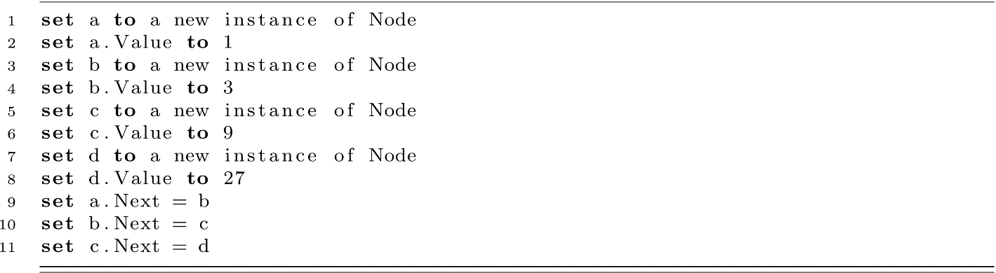

Figure 5.3
Operations on Linked Lists
Lookup (List Traversal)
Continuing the comparison with arrays, our first task will be to look up the value at an arbitrary position relative to a particular node in a linked list. You may consider a position in a linked list as the analogue of an array’s index. It is the ordinal number for a specific value or node within the data structure. For the sake of consistency, we will use 0-based positions.
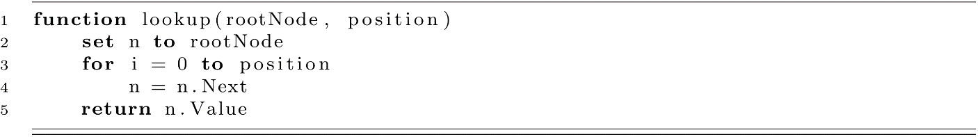
We address lookup first because it most clearly illustrates the means by which we traverse the linked list. On line 2, we start with some node, then lines 3 and 4 step forward to the next node an appropriate number of times. Whenever we wish to insert, delete, or look up a value or simply visit each node, we must either iteratively or recursively follow the Next reference for the desired number of sequential nodes.
Now that we have a means of looking up a value at an arbitrary position, we must consider how it performs. We start again by considering arbitrary index lookups in arrays. Recall that a lookup in an array is actually a single dereference of a memory address. Because dereferencing on an array is not dependent on the size of the array, the runtime for array lookups is O(1). However, to look up an arbitrary element in a linked list (say, the nth element), we must dereference n − 1 different addresses as we follow the Next reference. We now have a number of dereferences dependent on the length of the linked list. Specifically, our cost function of the worst-case scenario will be f(n) = n − 1, where n is the length, which is clearly O(n). Dereferencing within some loop or with recursion is a featured pattern in nearly every linked list algorithm. Therefore, in most cases, we will expect these algorithms to run in O(n) time.
Length (and Additional Means of Traversal)
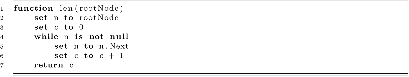
While it is the case that most list traversals are implemented with for-loops, there are occasions where other styles of traversal are more appropriate. For example, for-loops are ill-suited for scenarios where we do not know exactly how many times we must loop. As a result, while-loops are often used whenever all nodes must be visited. Consider the function below, which returns an integer representing the number of elements in the list starting at rootNode:
Also worth noting is that, due to the self-referencing definition of the Node class, many list procedures are reasonably implemented using recursion. If you consider a given root node, the length of a linked list starting at that node will be the sum of 1 and the length of the list starting at the Next reference (the recursive case). The length of a list starting with a null node is 0 (the base case).
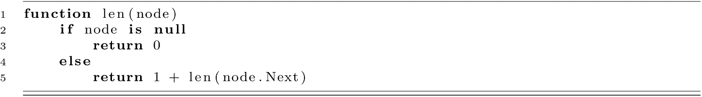
As we explore more algorithms in this book, we will discover that often recursive solutions drastically reduce the complexity of our implementation. However, we should pay close attention here. Because we dereference the Next node for every node visited, our solution still runs in O(n) time.
Insert
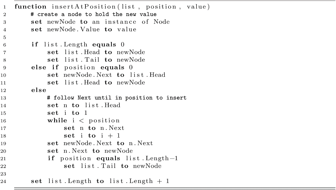
To create a general-purpose data structure, our next operation will be to insert new values at arbitrary positions within the linked list. For the sake of simplicity, this function assumes that the position is valid for the current length of the linked list.
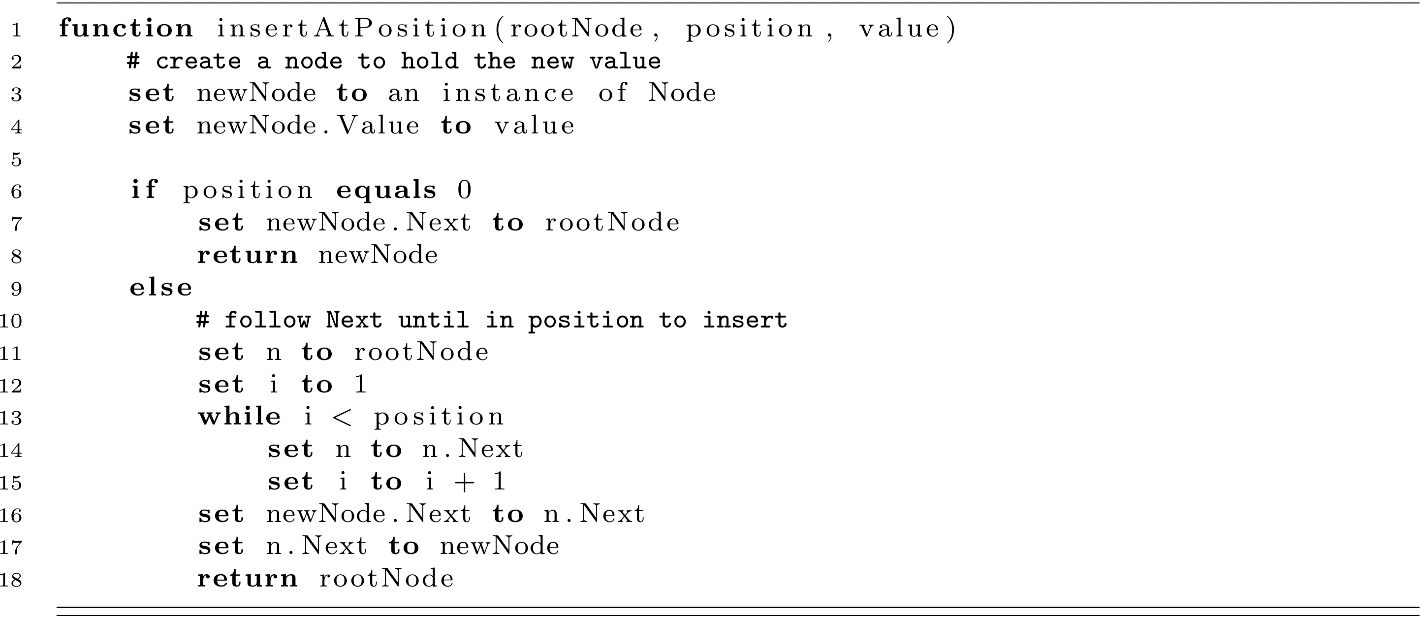
When reading and trying to comprehend this algorithm, we should pay close attention to three key things:
- We again see a linear traversal through the list to a given position by traversing the Next reference. As usual, it does not matter whether this is achieved with a for-loop, a while-loop, or recursion, the result is still the same. We maneuver through a list by starting at some point and following the references to other nodes. This is an incredibly important concept, as it lays the foundation for more interesting and useful data structures later in this book.
- When implementing algorithms, edge cases sometimes require specific attention. This function is responsible for inserting the value at a desired position, regardless of whether that position is 0, 2, or 200. Inserting a value into the middle of a linked list means that we must set references for the prior’s Next as well as newNode.Next. Inserting at position 0 is fundamentally different in that there is no prior node.
- More so than other statements, lines 14 and 15 may feel interchangeable. They are not. Much like the classic exchange exercise in many programming textbooks, executing these statements in the reverse order will lead to different behavior. It is a worthwhile exercise to consider what the outcome would be if they were switched.
We can visually trace the following example of an insertion:
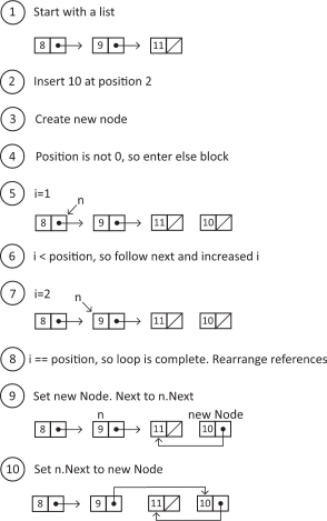
Figure 5.4
Next, we come to the runtime analysis of this function. Due to the linear traversal, we consider the algorithm itself to be of O(n) regardless of whether we are inserting at position 2 or 200. However, what if we want to insert at position 0? In this case, the number of operations required is not dependent on the length of the linked list, and therefore this specific case runs in O(1). When studying algorithms, we typically categorize using the worst-case scenario but may specify edge-case runtimes when appropriate. In other words, if we only ever care about inserting at the front of a linked list, we may consider this special case of insert to be an O(1) operation.
Remove
Now that we have seen how to traverse the list via the Next reference and rearrange those references to insert a new node, we are ready to address removal of nodes. We will continue to provide the root node and a position to the function. Also, because we might choose to remove the element at the 0 position, we will continue to return the root node of the resulting list. As with the insertAtPosition, we assume that the value for position is valid for this list.
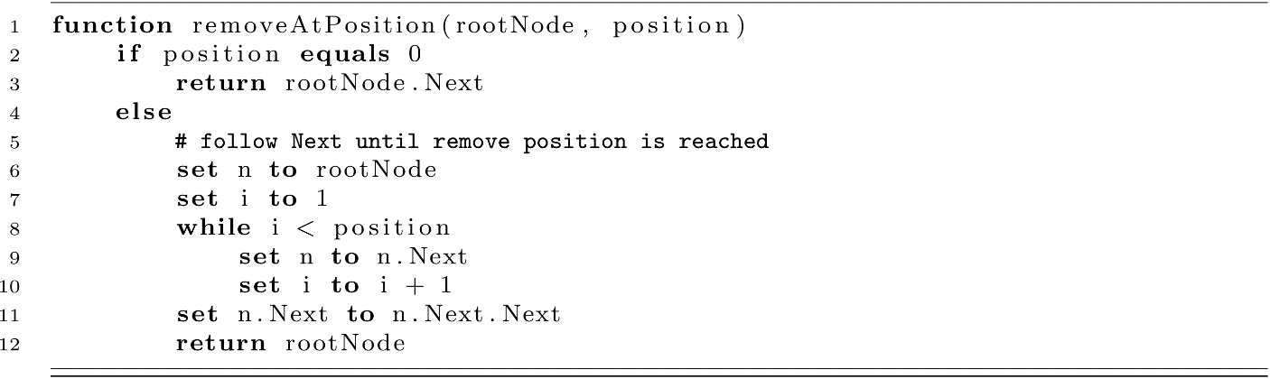
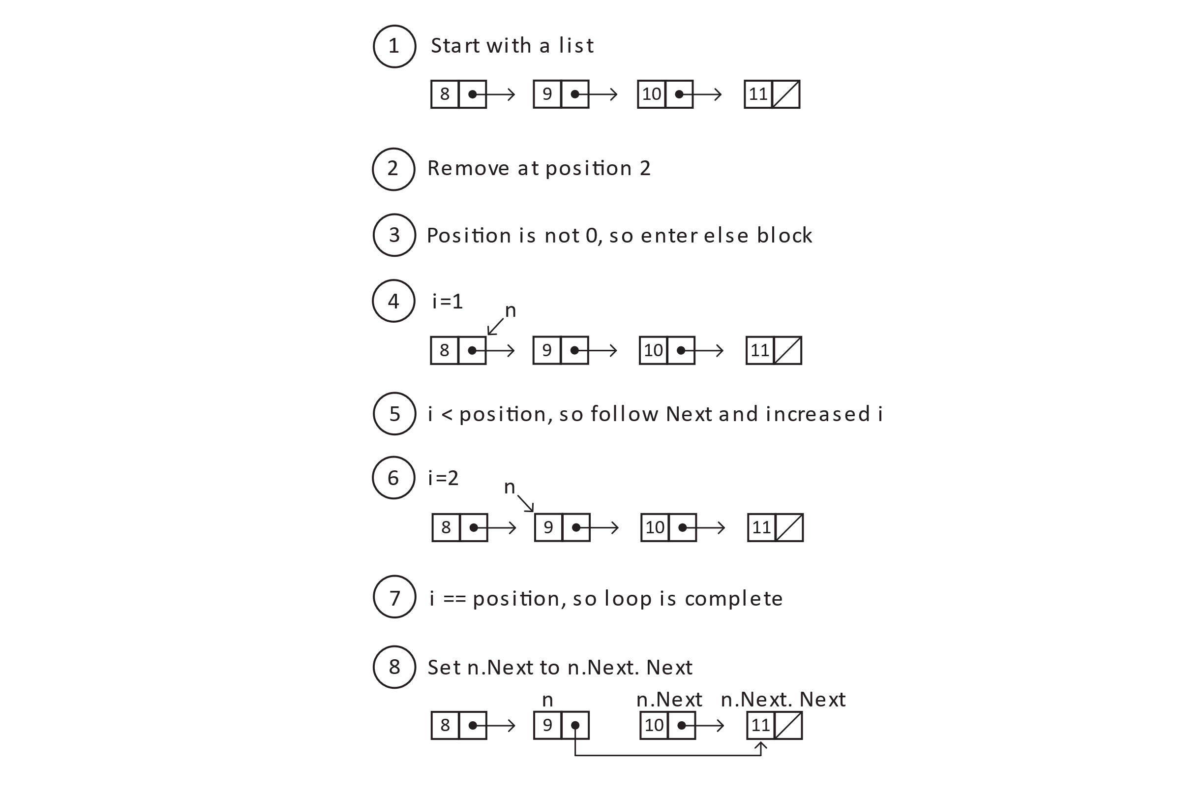
Figure 5.5
The result of the diagram above is that a traversal of the linked list will indeed include the values 8, 9, and 11 as desired. We should pay close attention to the node with value 10. Depending on the language we choose to implement linked lists, we may or may not be required to address this removed node. If the language’s runtime is memory managed, you may simply ignore the unreferenced node. In languages that rely on manual memory management, you should be prepared to deallocate the storage. The runtime for the algorithm, as a function of the length of the list, is still O(n), with the special case of position as 0 running again in constant time.
Doubly Linked Lists
Consider a scenario where we want to track the sequence of changes to a shared document. Compared to arrays, a linked list can grow as needed and is better suited for the task. We choose to inspect the change at position 500 in the linked list at a cost of 499 dereferences. We then realize we stepped two changes too far. We are actually concerned with change 498. We must then incur a cost of 497 dereferences to simply move backward two steps. The issue is that our nodes currently only point to the next value in the sequence and not the previous. Luckily, we can simply choose to include a Prior reference.
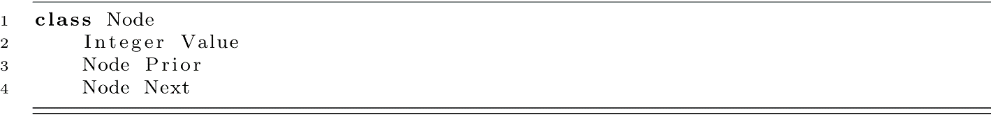
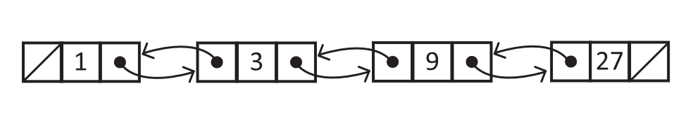
Figure 5.6
The choice to track prior nodes in addition to the next nodes does come with trade-offs. First, the size of each node stored is now larger. If we assume an integer is the same size as a reference, we have likely increased the size of each node stored by 50%. Depending on the needs of the application, constraints of the physical device, and size of the linked list, this increase may or may not be acceptable.
We also have more complicated (and technically slightly slower) functions for insertion and removal of nodes. See the pseudocode below for considerations in the general case. The case when position is 0 has also been omitted. Completing that case is an exercise at the end of this chapter.
Reference Reassignment for Singly Linked List Insert

Reference Reassignment for Doubly Linked List Insert
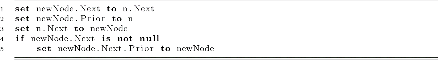
If we would like to make use of a Prior reference, we now must maintain that value on each insertion and removal. At times it is as easy as setting a value on an object (line 2). Other times we have to introduce a new condition (line 4). In this case, we check newNode.Next against null because we may be inserting our new value at the end of the list, in which case, there will not be any node with Prior set to newNode. Doubly linked list insert now requires as many as 5 operations where we only had 2 for singly linked lists. While this does mean that doubly linked list insert is technically slower, we only perform these operations once per function call. As a result, we have two functions that run in O(n) even though one is technically faster than the other.
Returning to the change tracking example at the beginning of this section, we now have a means of moving forward and backward through our list of changes. If we wish to start our analysis of the change log at entry 500, it will indeed cost us 499 dereferences to reach that node. However, once at that node, we can inspect entry 498 with a cost of 2 dereferences by following the Prior reference.
Augmenting Linked Lists
Just as we saw when inserting or removing at position 0, we can often find clever ways to improve certain behaviors of linked lists. These improvements may lead to better runtimes or simply have a clearer intent. In this section, we will consider the most common ways linked lists are augmented. Generally speaking, we will follow the same strategy used for doubly linked lists. The main principle is this: At the time that we know some useful bit of information, we will choose to simply save it for later. This will lead to a marginally higher cost for certain operations and a larger amount of data to store, but certain operations will become much faster.
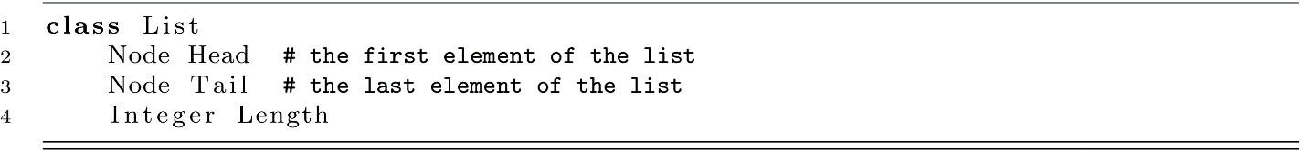
So far in this chapter, we have implicitly defined a list as a single node representing the root element. To augment our data structure, we will now more formally define the full concept of a list as follows. For the definition of this class, we can choose to use a singly or doubly linked node. For simplicity, examples in this section return to using a singly linked node.
As was the case with doubly linked lists, our insert and remove code is now substantially more complicated. One nice benefit is that we now modify the list object and no longer need to return the root node.
For each insert into the list, we must now maintain some new values on the list object. Lines 7, 8, 11, and 22 help keep track of when we have changed the head or tail of the list. Line 24 runs regardless of where the value was inserted because we now have one more element in the list.
This extra work was not in vain. Consider what was required if we wanted to write a function to return the last element of a linked list represented by the root node compared to running it on a list object.
Last Element Using Root Node and Next References
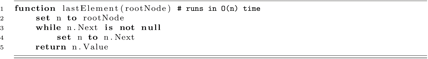
Last Element Using the List and Tail References

The same improvements can be seen in retrieving the length of a list.
Length Using Root Node and Next References
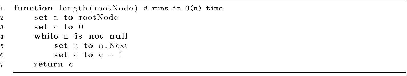
Length Using the List and Length Values

Abstract Data Types
Before closing this chapter on linked lists, we benefit from considering abstractions. An abstract data type (ADT) is a collection of operations we want to perform on a given data type. Just as we can imagine numerous implementations for a given data structure (maybe we change a for-loop to a while-loop or recursion), we can also imagine numerous data structures that satisfy an ADT.
Consider the operations defined above for linked lists. We often want to insert, delete, count, and iterate over list elements. We call this set of operations a list ADT. A list may be implemented using linked nodes, an array, or some other means. However, it must provide these four operations. Implied in this description of ADTs is the fact that we cannot discuss the asymptotic runtime or space requirements of an ADT. Without knowing how the ADT is implemented, we cannot conclude much (if anything) about the runtime. For example, we could conclude that iteration is no better than O(n) because iteration requires us to touch each element regardless of implementation. We could not determine anything about the runtime of lookup because an array would be O(1), a linked list O(n), and a skip list O(log n). This last data structure is not formally covered in this chapter.
In subsequent chapters, we will at times refer to ADTs without specifying the precise data structure. In doing so, we will be able to focus on the new data structure without concern for how the ADT is implemented. Naturally, when we address the runtimes and space utilization of those algorithms, we must choose between data structures.
Exercises
- Write three functions that print all values in a singly linked list. Write one using each of the following: for-loop, while-loop, and recursion.
- Write a removeAtPosition function for a doubly linked list that correctly maintains the Prior reference when the removal occurs at position 0, length − 1, or some arbitrary position in between.
- Write a removeAtPosition function for a singly linked list that correctly maintains the Head and Tail references when the removal occurs at position 0, length − 1, or some arbitrary position between.
References
Cormen, Thomas H., Charles E. Leiserson, Ronald L. Rivest, and Clifford Stein. Introduction to Algorithms, 2nd ed. Cambridge, MA: The MIT Press, 2001.
