Introduction

We begin by listing some desirable aspects of data structures:

• economical and dynamic memory consumption
• ability to insert or delete keys in sublinear time
• ability to look up keys by exact match to a key in sublinear time
• ability to retrieve several key values based on a range

With these criteria in mind, let us review some of the data structures studied so far. Arrays allow us constant-time lookup, assuming we know the index of the item we want to retrieve. Finding that index requires a linear traversal of an unsorted array or a logarithmic Binary Search of a sorted array. Arrays have an unfortunate side effect in that they must be preallocated in memory. As a result, inserts and deletes require either excess allocation or reallocation (with a great deal of copying).

We then considered linked lists. Conveniently, we are not required to know the capacity before performing the initial insert. Linked lists are less economic in memory consumption, as each stored datum requires us to also store a next (and possibly previous) reference. Locating a particular position for insert or delete requires a Linear Search, but the insertions or deletions at that point are constant time.

Then we arrived at hash tables. Finally, we had a data structure that allowed for true constant-time lookups based on a key. Inserts and deletes were also constant-time operations, assuming a sufficient hash function. These improvements were substantial but left us no option for retrieval of values based on a range.

What we want is some general-purpose data structure that maximizes the desired utility of linked lists while minimizing the rigidity of arrays and hash tables. Binary search trees fit nicely into this niche. Reusing some concepts we have learned so far, we can achieve sublinear times for inserts, deletions, and retrievals. We can grow and shrink our size as needed. We will require more storage than arrays but will not require the excess capacity as with hash tables.

Brief Introduction to Trees

Binary search trees are a subclass of binary trees, which are a subclass of trees, which are a subclass of graphs. Here we will only introduce enough details to facilitate an understanding of binary search trees. In chapter 11, we will provide more precise mathematical definitions of graphs and trees.

Trees (as well as graphs in general) consist of nodes and edges. As a note, nodes are also referred to as vertices (or vertex in the singular form). We will use nodes as containers for data, such as an integer, string, or even a database record. Nodes are related to other nodes via edges. Each edge connects two nodes and describes the relationship between those nodes. Edges in binary trees are child/parent relationships. One node is the parent, and the other is a child. Each node has at most one parent. A tree will have exactly one node without a parent. This node is called the root. Each node has no more than two children. A node with zero children is called a leaf. From time to time, we may consider a subtree, which is any given node and all its descendants. Although this chapter will focus mainly on binary trees, you should note the term “m-ary tree,” where m is any positive integer and represents the maximum number of children for any given node.

Now we consider some additional tree-related terms. It is important to note that these terms are not consistently defined across different textbooks. In order to be consistent with another source you may likely read (Wikipedia), I will defer to the definitions found there. Whenever reading a new text, ensure that you first review that source’s definition of terms:

• height—the number of nodes from a leaf node to the root, starting at 1
• depth—the number of nodes from the root to a particular node, starting at 1
• level—all descendants of the root that have the same depth
• full—a given m-ary tree is full if each node has exactly 0 or m children
• complete—a given m-ary tree is complete if every level is filled except possibly the last (which is filled from left to right)
• perfect—a given m-ary tree is perfect if it is full and all leaf nodes are at the same depth

Below is an example of a tree. Interior nodes are gray, and leaf nodes are white. The root node has been marked with an “R.” Note that this is a ternary tree because any given node has at most three children. It is not full, which implies that it is neither complete nor perfect.

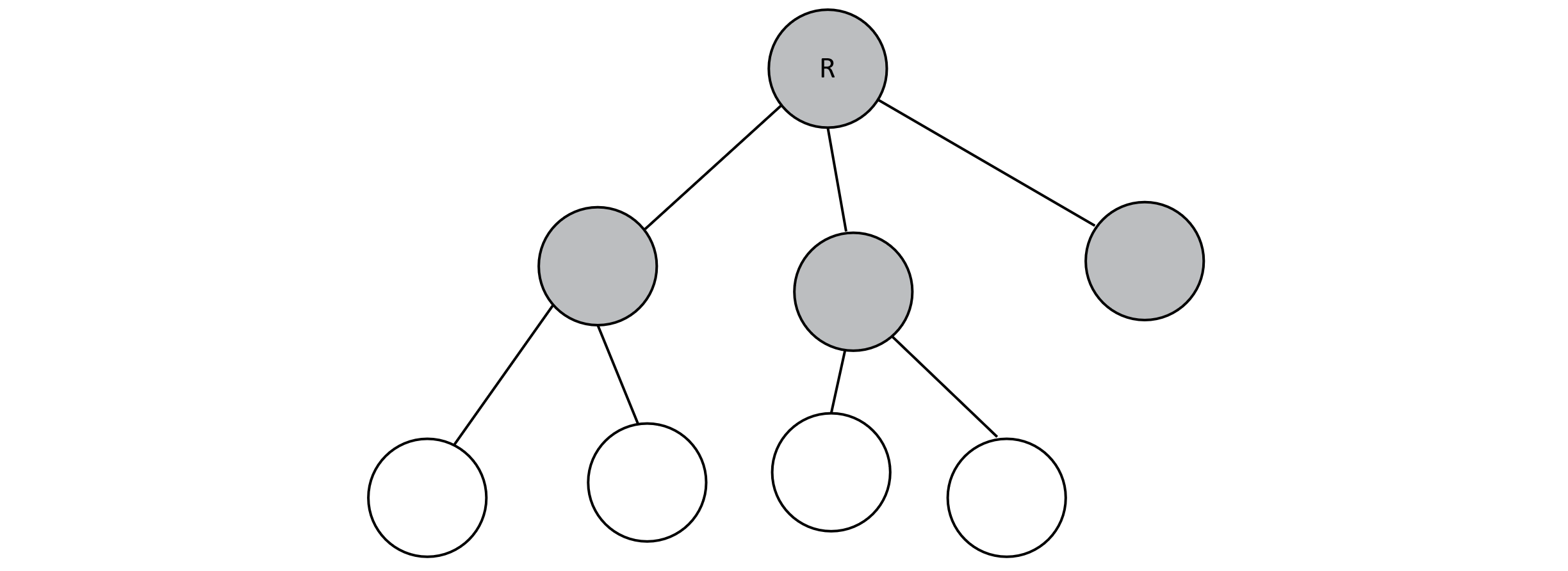
Figure 8.1

We may now make some useful assertions regarding binary trees:

• Because a perfect binary search tree implies that every interior node has two children, the number of nodes (n) is 2^k − 1, where k is the number of levels in the tree. In a related manner, the number of levels in a tree is the floor of log₂ n.
• Of all nodes in a perfect binary search tree, roughly half are leaf nodes, and the other half are interior. Precisely, the number of leaf nodes will be the ceiling of n/2, and the number of interior nodes will be the floor of n/2.

So far this concept of a tree does not produce much benefit. We could assign a key to each node, but what exactly would that mean? What does the relationship between parent and child imply? To derive value from trees, binary trees are insufficient, and we must apply more constraints.

A binary search tree (BST) is a specific type of binary tree that ensures that

• each node (N) is assigned a key.
• each node has a left child (L), which represents the subtree rooted at node L. The key of every node in this subtree is less than the key stored in node N. It is possible that a given node has no left child.
• each node has a right child (R), which represents the subtree rooted at R. The key of every node in this subtree is greater than the key in node N. It is possible that a given node has no right child.

Figure 8.2 is an example of a BST. The key stored in each node is an integer but could be of any data type that can be sorted. For convenience, we are assuming that BSTs do not contain duplicate keys, although we do not exactly need to. The tree below is perfect, but a BST does not need to be. As we discuss BSTs further, we will start to consider more problematic configurations.

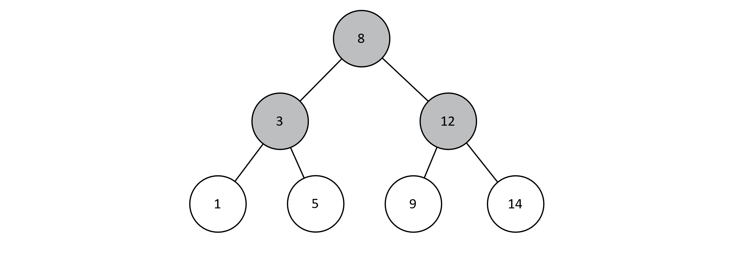
Figure 8.2

To understand the structure of a BST better, we can consider an in-order traversal of the tree. This traversal is one in which we recursively visit the left child, current node, and right child. If you were to print each key during an in-order traversal, the result would be all keys from the tree in ascending order.

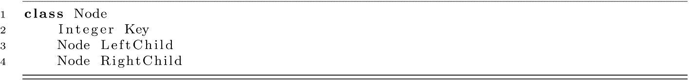
As implied in the figure above, nodes are modeled using the following class. In most practical applications, the Key property would hold some data other than type integer. Regardless, the simplicity of this model will be useful for the remainder of the chapter.

Searching

Searching is a simple operation. You begin at the root node considering a key (x) you want to find. If the key stored at the node is x, you have found it. If x is less than the node’s key, you search the left subtree. If x is greater than the node’s key, you search the right subtree. You continue this process until you arrive at a leaf node and have no more children to consider. Below is the pseudocode to further clarify the algorithm. The function is originally called with the root node, which then changes to descendants in the recursive calls.

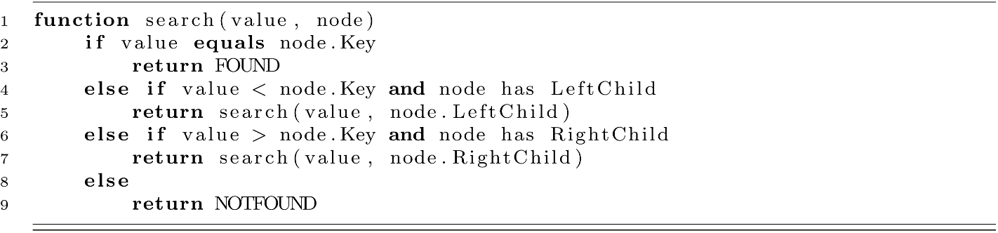
Next, we should consider the runtime of searching a BST. Just as with searching arrays and linked lists, we want to consider the amount of work necessary as the size of the data structure increases. In our recursive example above, we perform between 1 and 5 comparisons on each call to search (depending on exactly how you count). As a result, we have no more than 5 comparisons for each node visited. Because 5 is not dependent on the overall number of nodes, the amount of work to perform for each node visited is constant with respect to n.

How many nodes must we visit in the worst-case scenario? If we compare the desired value to the key at the root node and do not find the value, we have immediately eliminated roughly half of the values in our tree. Once at the second level, we perform the comparison again and eliminate half of this subtree, which was in turn half of the original. As a result, we reduce the number of keys we have to consider by half each time we visit a child. At worst, we will have to visit only one node in each level of the tree, resulting in ceiling log₂ n nodes visited. With O(log n) nodes visited and O(1) amount of work at each node, search can be run in O(log n) time for a perfect BST.

Insertion

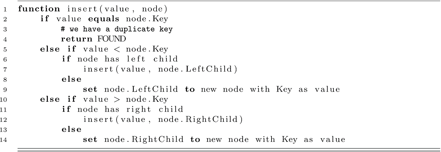
To this point, we have assumed that a BST exists. We have yet to create one. Insertion simply searches for a valid position where the key would be if it existed and adds it at that position. In other words, the search for a nonexistent key always terminates in a leaf node. A naïve insertion algorithm considers this leaf node. If the key to insert is less than the leaf’s key, you insert a new node as the left child. If the new key is greater than the leaf’s key, you insert it as the right child. Pseudocode is included below to clarify:

Deletion

When possible, it is good practice to enumerate the possible states that an algorithm may have to consider. When deleting a key from a BST, the node containing that key may be in four different states with respect to its children: no children, left child only, right child only, and both left and right children.

No Children

First, we must locate the node containing the key to be deleted. If that node has no children, it is by definition a leaf node. To delete a key at the leaf node, it suffices to simply remove the parent’s reference to the leaf node. In the example below, the node containing the value 4 has no children. We can simply go to that node’s parent and set the left child reference to null.

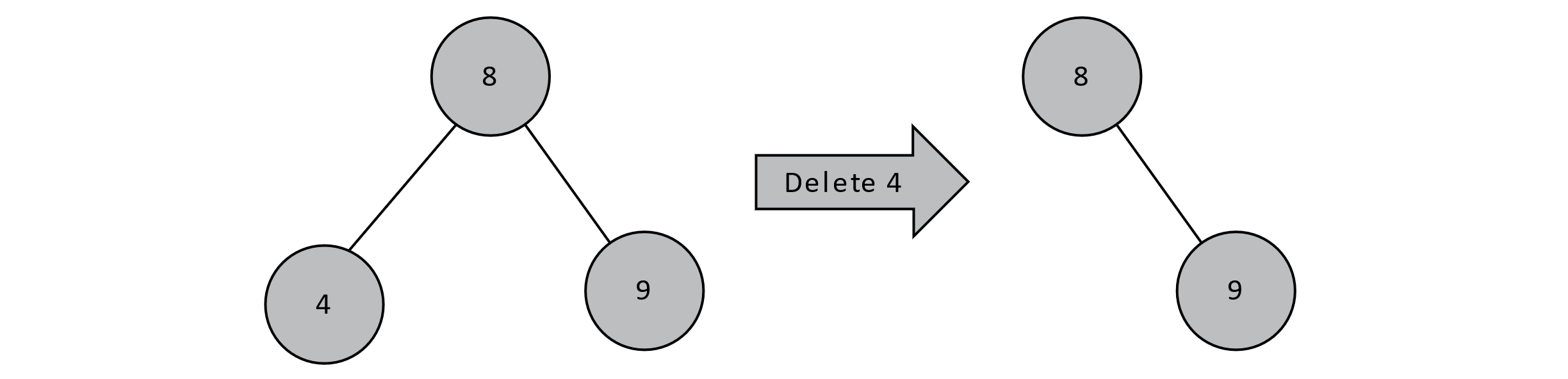
Figure 8.3

Left Child Only / Right Child Only

If a node contains a key to be deleted and has only one child, we can shift the appropriate subtree up. We can do this because all descendants in a node’s left subtree are less than that node’s value. In the case below, all left-side descendants of 8 are nodes containing values less than 8. If 4 only has one child, we can simply promote that child by setting 8’s left child to that node. Similar reasoning would apply if 4 only had a right child.

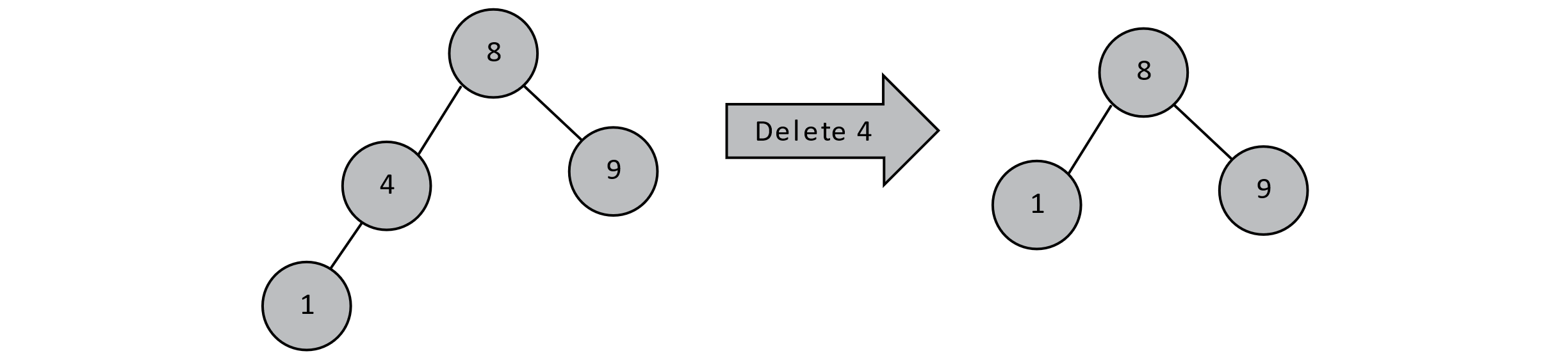
Figure 8.4

Both Left and Right Children

If a node containing a value to be deleted has both left and right children, we now must consider the possibility that those children may also be parents. This notably complicates the decision of what should be node 8’s left child. If we were to shift the subtree starting at 1 up to 8’s left child, that new node would have two right children (2 and 6), which obviously does not work. You would encounter a similar issue trying to promote 6 to be 8’s left child. What we need instead is to find 4’s in-order predecessor or in-order successor, remove that value from the tree (it is a leaf), and place it where 4 was. In the example below, we promoted 4’s in-order predecessor, but we could have just as easily promoted the value 5.

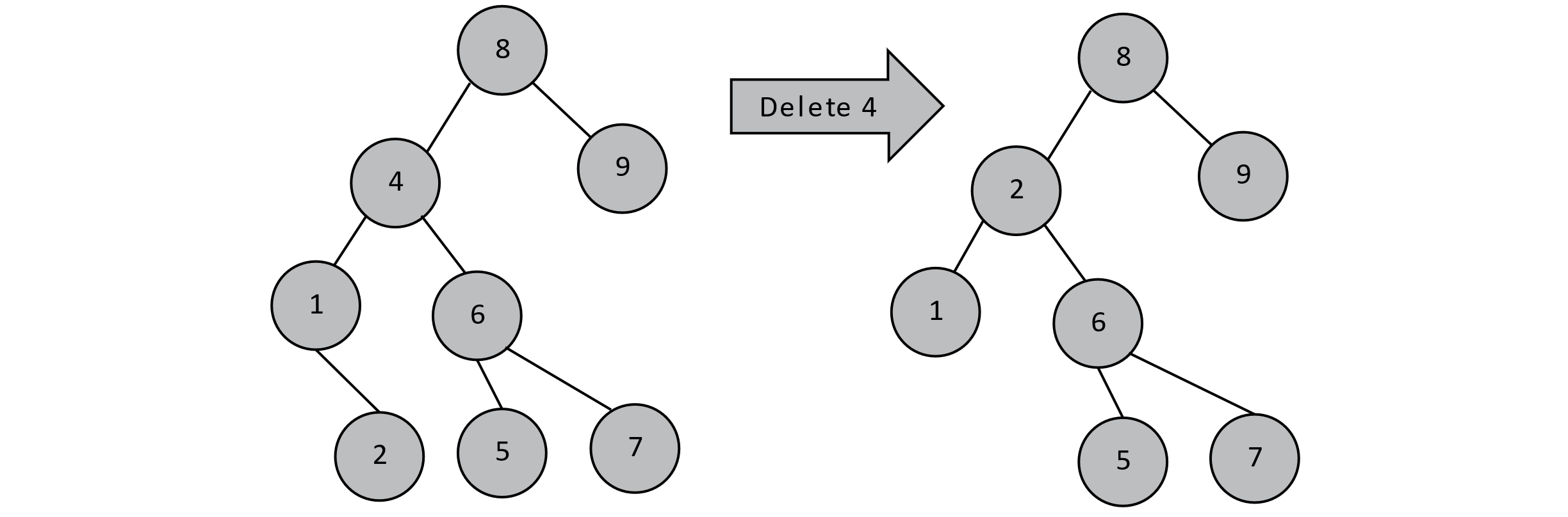
Figure 8.5

Unbalanced BSTs

When assessing the performance of search in BSTs, we had silently assumed that trees are perfect (or at least complete). We relied on this convenient property that the height of the tree was related to the logarithm of the number of nodes. In practice, this is rarely the case. Imagine we built a perfect BST using keys 1 through 7.

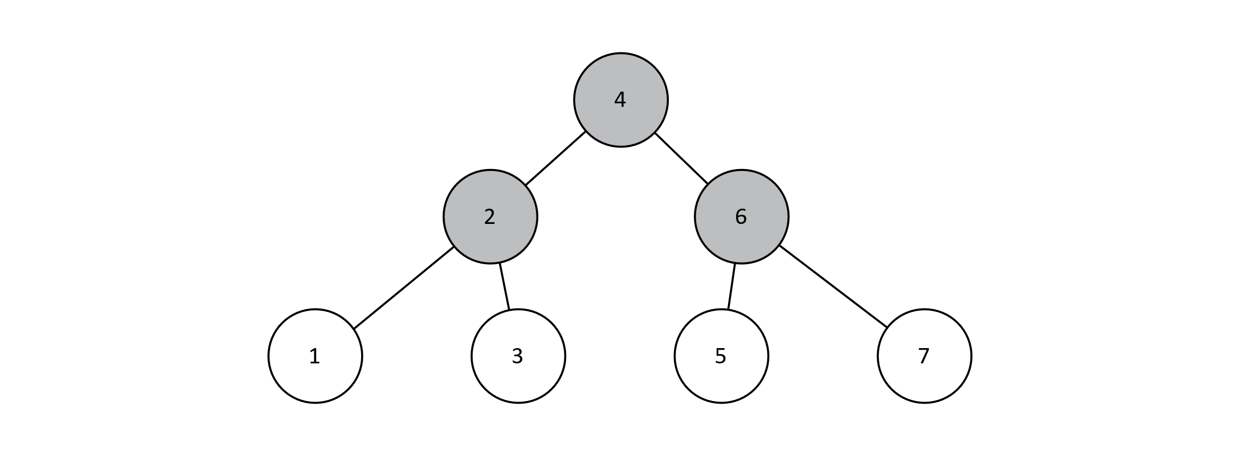
Figure 8.6

In figure 8.6, we can visualize the relationship between the number of nodes and the height of the tree. This relationship is logarithmic, so we can count on searching, inserting, and deleting keys to run in logarithmic time. However, if we perform inserts as specified above (in order from 1 to 7), we will actually end up with the tree in figure 8.7. Take a moment to trace the algorithm with pencil and paper to convince yourself this is the case.

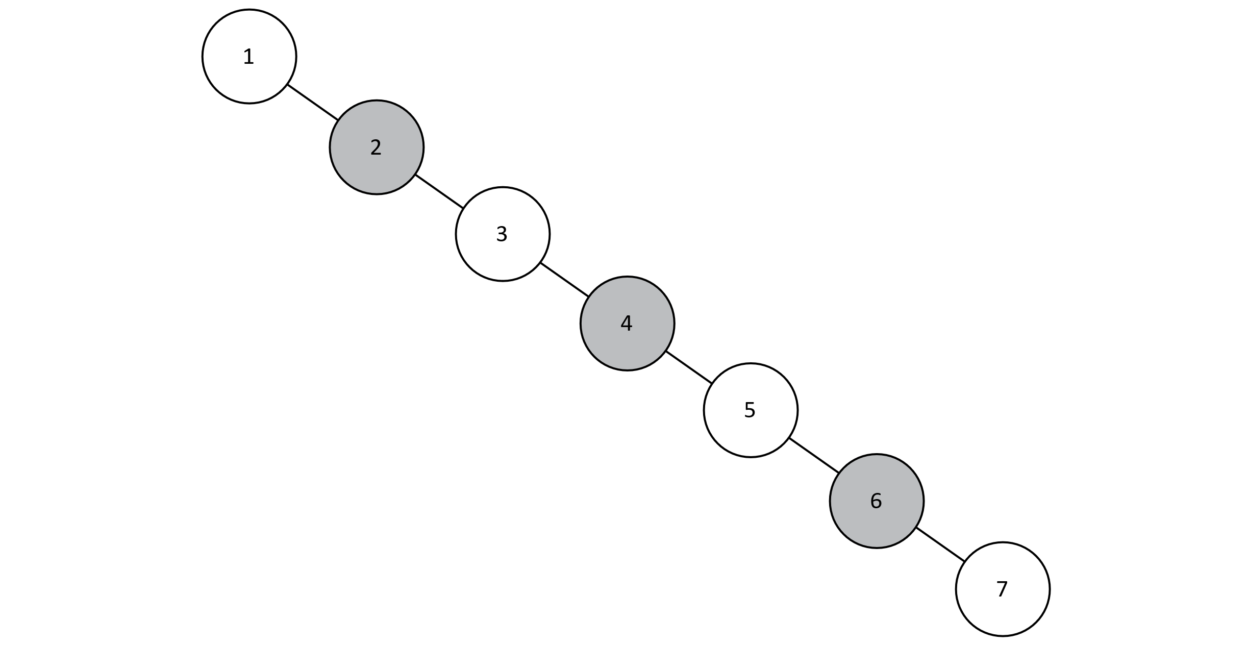
Figure 8.7

Our resulting structure, although technically a BST, also closely resembles a sorted linked list. When we studied linked lists, we were only able to search in linear time because all n nodes must be visited to ensure we found the desired key. The lesson learned is this: if we are not careful about how we perform inserts, we may likely construct a tree structure that cannot support O(log n) searches.

Ideally, we would love a tree to be perfect after each insert. This is not mathematically possible. If you have a perfect tree with seven nodes and three levels, inserting an eighth node will create a new level and result in a state where not all leaf nodes have the same depth. It may be desirable to maintain a complete tree. However, recall that complete trees must fill the lowest level from left to right. This constraint is not necessary, as we will be just as happy to fill it out right to left or in completely arbitrary order. As we can see, we need a new term to describe BSTs that allow for O(log n) searches and avoid the linked list type of configuration.

In a manner of speaking, we want our tree to be balanced after each insert. At this time, we will loosely define balance to be the condition such that the subtree heights of left and right subtrees are roughly equal. That leads to our next question: Can we modify our insert such that (1) the tree can remain balanced after each insert and (2) inserts can still be performed in O(log n) time?

Self-Balancing Trees

Self-balancing trees are those that maintain a balanced structure after each insertion and deletion and thus maintain an O(log n) search time. A thorough survey of these data structures could constitute chapters of text. This section will introduce how AVL trees maintain a balanced structure during insertion. We focus only on the insertion, but deletion must be addressed as well. Search, however, does not change from the naïve BST. Additional resources at the end of the chapter provide more information about this and other self-balancing trees.

AVL Trees

AVL trees are named after the computer scientists who developed them (G. M. Adelson-Velsky and E. M. Landis). After insertions that leave the tree in an unbalanced state, we achieve balance by performing small constant-timed adjustments called rotations.

First, we must determine whether an insertion has resulted in an unbalanced tree. To determine this, we use a metric called the balance factor. This integer is the difference in the heights of a node’s left and right subtrees. Below is the simplest possible tree where we can witness such an imbalance. As usual, values are stored inside the node. Subtree heights are stored at the upper right of each node. If a left or right child does not exist, then the subtree height is 0. In this example, the node containing 8 has a left child with subtree height of 2 and a right child with subtree height of 0. The absolute difference between 2 and 0 is 2. This is above our threshold of 1, so our tree is unbalanced.

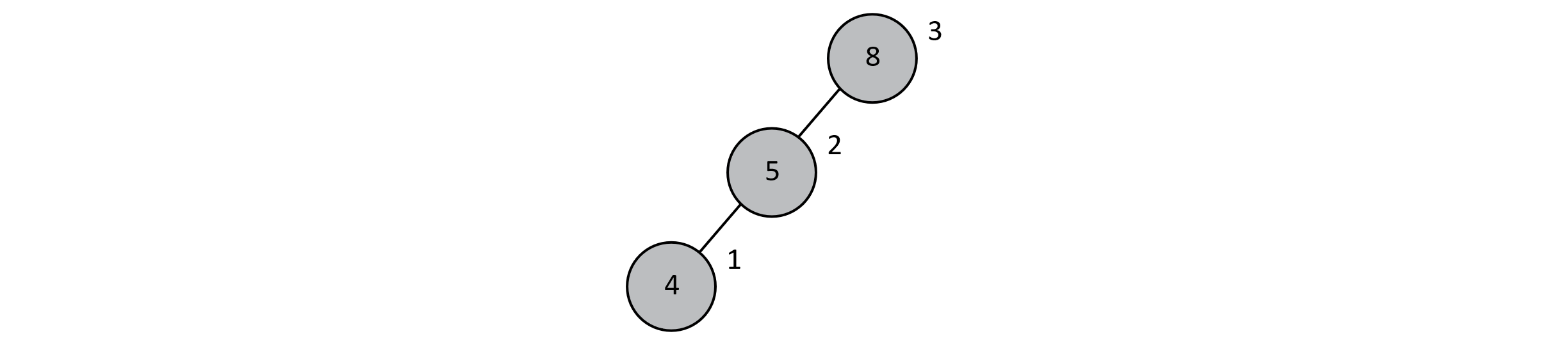
Figure 8.8

We now have a means for detecting unbalanced trees and are left to determine how to bring the tree back into balance. This is where we employ rotations. Rotations are small, constant-time adjustments to a subtree that improve the balance of that subtree. They are called rotations because they have the visual effect of rotating that subtree to a more balanced state. In figure 8.8, a rotation makes the 5 node the new root with a left child of 4 and a right child of 8. This is visually depicted in figure 8.9. Notice that after the rotation, the height of the subtree starting at 8 is now 1. Node 5 has left and right subtrees both at height 1. The difference is 0, which is not greater than 1, indicating that we are now in balance.

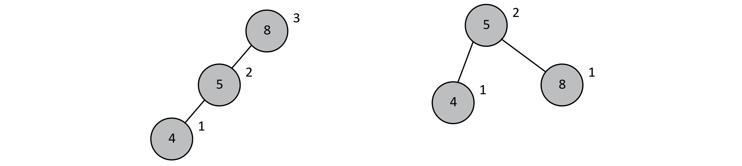
Figure 8.9

We make one last consideration regarding AVL trees. Earlier we had described this modification to BSTs as “self-balancing” and the heights of left and right subtrees as roughly equal. What actually happens is more nuanced and worthy of discussion. With perfect BSTs, we concluded that the relationship between the number of nodes in the tree and the number of comparisons required for a search was logarithmic. For AVL trees, we must be able to show the same relationship applies.

A proof by induction is able to show that the height of any AVL tree is O(log n). Note the distinction here. Perfect binary trees were shown to have a height equal to the ceiling of log₂ n (or more precisely, log₂(n+1)). AVL trees are said to have a height of O(log n), which is less precise. Rather than reviewing the inductive proof (which can easily be found online and in many reference textbooks), let us consider the following two trees:

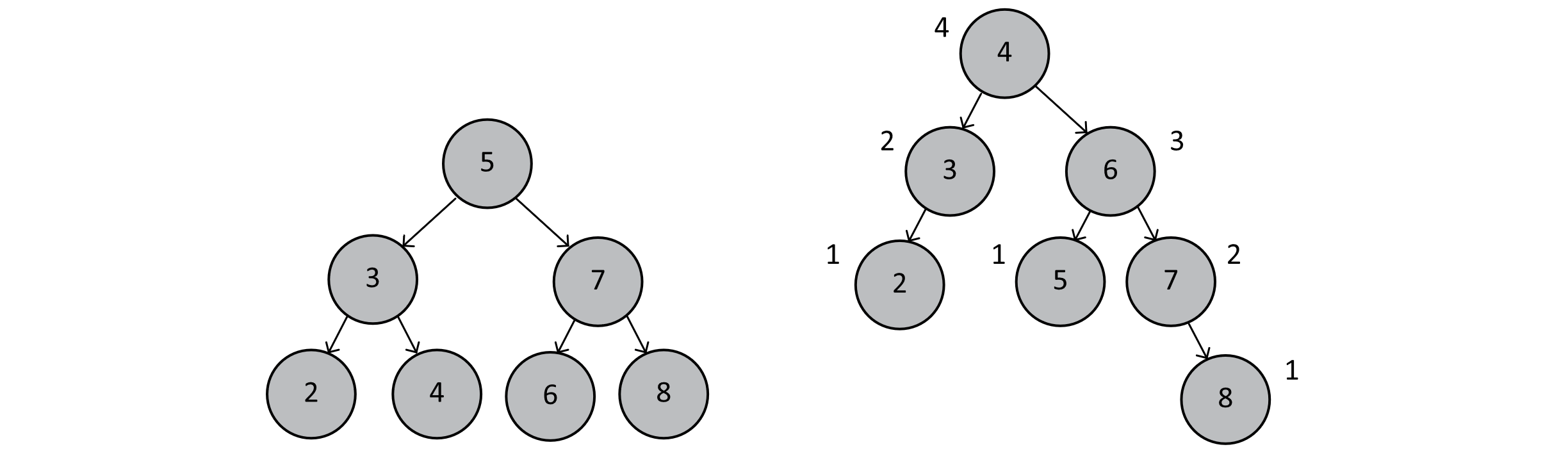
Figure 8.10

The tree on the left is a perfect BST. It has 7 nodes, which implies a height of log₂(7+1) = 3. The tree on the right is a balanced AVL tree. Note that the height is no longer 3, even though we claim that the tree is balanced and that search times are still O(log n). We point this out to illustrate that while some algorithms may share the same Big-O classification, their actual runtimes may differ. Because of the rotations, we ensure that the difference in heights of the left and right subtrees is no more than 1. This then ensures that our AVL tree, while not complete or perfect, has a height no greater than 1 + log₂(n+1). The additional 1 does not significantly impact the growth of the function as n becomes very large, so we can conclude that searching an AVL tree can still be accomplished in O(log n) time.

References

Alexander, Eric. “AVL Trees.” Computer Science User Pages. University of Wisconsin-Madison. Accessed September 27, 2023. https://pages.cs.wisc.edu/~ealexand/cs367/NOTES/AVL-Trees/index.html
“Binary Tree.” Wikipedia. Last modified August 28 2023. https://en.wikipedia.org/wiki/Binary_tree
Galles, David. “AVL Tree.” USF Computer Science Department. Accessed September 27, 2023. https://www.cs.usfca.edu/~galles/visualization/AVLtree.html
Galles, David. “Binary Search Tree.” USF Computer Science Department. Accessed September 27, 2023. https://www.cs.usfca.edu/~galles/visualization/BST.html