Introduction

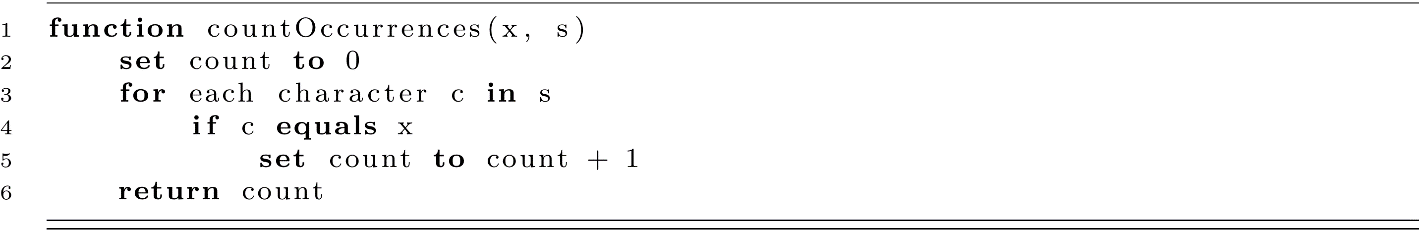
As a student of computer science, you have already accomplished a broad array of programming tasks. In order to fully understand where we are going, let us first consider where we have been. We will start by analyzing a programming exercise from an introductory class or textbook. Consider a function that counts the occurrences of a particular character x within a string s.

With regard to learning a programming language, this exercise serves many purposes. In order to solve this problem, you must first understand various features of a language’s syntax:

• Variables are units of data that allow us to store intermediate results.
• Iteration is a means of systematically visiting each element in a sequence.
• Conditionals allow us to choose whether to execute a particular set of statements.
• Functions allow us to encapsulate logic and reuse it elsewhere.

Individually, each of these concepts is neither interesting nor impactful. The real power in computation comes from combining these into meaningful solutions, and in that combination lies the purpose of this text. Moving forward, we will refer to this combination of elements as synthesis.

Synthesis is something we learn to do through the study of data structures and algorithms. These are known and well-researched solutions. This text will require us to learn the patterns and trade-offs inherent in those existing solutions. However, there is a blunt truth underlying this course of study: you will likely never implement these algorithms or data structures again. This leads to the obvious question of “Why study them in the first place?” The answer lies in the imminent transition from skills to synthesis.

Synthesis is hard, regardless of your field of study. Arithmetic, algebra, and geometry are relatively easy compared to engineering. Performing at a piano recital is not the same as composing the music. Basic spelling and grammar are not sufficient for writing a novel. Writing a conditional or loop is inherently different than creating software. There is one major difference: arithmetic, piano, and grammar all have utility outside of synthesis. There is no utility in this world for conditional statements and loops if you cannot apply them to solve new problems.

For many students, this transition from programming skills to synthesis of solutions will require significant effort. It is likely that you have experienced nothing like it before. For that reason, we choose to “stand on the shoulders of giants” to see how others have transformed simple components into elegant solutions. This will likely require us to memorize much of what we see. You may even, from time to time, be asked to recall specific details of a data structure or algorithm. However, if your study of these solutions ends there, you have certainly missed the mark.

Consider another analogy. Bootstrapping is a computing technique employed when a computer loads a program. Rather than loading all instructions needed to execute a task, the computer loads only a small number of critical instructions, and those in turn load other instructions. In a sense, the program starts out with only a seed containing the most crucial, fundamental, and useful pieces of information. That seed does not directly solve any problem but rather solves a problem by acquiring other instructions that can. The study of data structures and algorithms will bootstrap your problem-solving skills. You may or may not explicitly use anything you learned, but the ideas you have been exposed to will give you a starting point for solving new and interesting problems later.

What Is a Data Structure?

Data encountered in a computer program is classified by type. Common types include integers, floating point numbers, Boolean values, and characters. Data structures are a means of aggregating many of these scalar values into a larger collection of values. Consider a couple of data structures that you may have encountered before. The index at the end of a book is not simply text. If you recognize it as structured data, it can help you find topics within a book. Specifically, it is a list of entries sorted alphabetically. Each entry consists of a relevant term followed by a comma-separated list of page numbers. Likewise, a deck of playing cards can be viewed as another data structure. It consists of precisely 13 values for 4 different suits, resulting in 52 cards. Each value has a specific meaning. If you wish to gain access to a single card, you may cut the deck and take whatever card is on top.

With each data structure encountered, we consider a set of behaviors or actions we want to perform on that structure. For example, we can flip over the card on the top of a deck. If we combine this with the ability to sequentially flip cards, we can define the ability to find a specific card given a deck of unsorted playing cards. Describing and analyzing processes like these is the study of algorithms, which are introduced in the next section and are the primary focus of this text.

What Is an Algorithm?

An algorithm is an explicit sequence of instructions, performed on data, to accomplish a desired objective. Returning to the playing card example, your professor may ask you to hand him the ace of spades from an unsorted deck. Let us consider two different procedures for how to accomplish this task.

The above is a meaningful illustration and represents our first encounter with the challenge of synthesis introduced in the first section of this chapter. When someone new to computer science is asked to find a card from a deck, the procedure more often resembles A rather than B. Whether working with cards in a deck or notes from class, our human brains can have the ability to process a reasonably sized set of unstructured data. When looking for a card in a deck or a topic in pages of handwritten notes, informal procedures like A work fine. However, they do have limitations. Procedure A lacks the precision necessary to guide a computer in solving the problem.

Algorithms and Implementations

From a design perspective, it makes sense to formulate these instructions as reusable procedures or functions. The process of reimagining an algorithm as a function or procedure is typically referred to as implementation. Once implemented, a single well-named function call to invoke a specific algorithm provides a powerful means of abstraction. Once the algorithm is written correctly, future users of the function may use the implementation to solve problems without understanding the details of the procedure. In other words, using a single high-level procedure or function to run an algorithm is a good design practice.

Expression in a Programming Language

If you are reading this book, you have at least some experience with programming. What if you are asked to express these procedures using a computer program? Converting procedure A is daunting from the start. What does it mean to spread the deck out on the table? With all “cards” strewn across a “table,” we have no programmatic way of looking at each card. How do you know when you have found the ace of spades? In most programming languages there is no comparison that allows you to determine if a list of items is equal to a single value. However, procedure B can (with relative ease) be expressed in any programming language. With a couple of common programming constructs (lists, iteration, and conditionals), someone with even modest experience can typically express this procedure in a programming language.

The issue is further complicated if we attempt to be too explicit, providing details that obscure the desired intent. What if instead of saying “Then hand him the card,” you say, “Using your index finger on the top of the card and your thumb on the bottom, apply pressure to the card long enough to lift the card 15 centimeters from the table and 40 centimeters to the right to hand it to your professor.” In this case, your instructions have become more explicit, but at the cost of obfuscating your true objective. Striking a balance between explicit and sufficient requires practice. As a rule, pay attention to how others specify algorithms and generally lean toward being more explicit than less.

Analysis of Algorithms

Constraints

How much work does it require to find the ace of spades in a single deck of cards? How many hands do you need? An algorithm (such as procedure B) will always be executed in the presence of constraints. If you are searching for the ace of spades, you would probably like your search to terminate in a reasonable amount of time. Thirty seconds to find the card is probably permissible, but four hours likely is not. In addition, finding the card in the deck requires manipulation of the physical cards with your hands. If you had to perform this task with one hand in your pocket, you likely would have to consider a different algorithm.

Constraints apply in the world of software as well. Even though modern CPUs can perform operations at an incredible rate, there is still a very real limit to the operations that can be performed in a fixed time span. Computers also have a fixed amount of memory and are therefore space constrained.

Scalability

A primary focus in the study of algorithms is what happens when we no longer have a single deck of 52 cards. What if we have a thousand decks and really bad luck (all 1,000 aces of spades are at the back of the deck)? No human hands can simultaneously hold that many cards, and even if they could, no human is going to look at 51,000 other cards to check for an ace of spades. This illustrates the desire for algorithms to be scalable. If we start with a problem of a certain size (say, a deck of 52 cards), we particularly care about how much harder it is to perform the procedure with two decks. With a large enough input, any algorithm will eventually become impractical. In other words, we will eventually reach either a space constraint or a time constraint. It is therefore necessary that realistic problem sizes be smaller than those thresholds.

Measuring Scalability

Measuring scalability can be challenging. It seems obvious (but worth noting) that a given algorithm for sorting integers may be able to sort 10 trillion values on a distributed supercomputer but will likely not terminate on a mobile phone in a reasonable amount of time. This means the simple model for measuring scalability (namely, how long an algorithm takes to run) is insufficient. Comparing algorithms without actually running them on a physical machine would be useful. This is the main topic of this section.

If we wish to analyze algorithm performance without actually executing it on a computer, we must define some sort of abstraction of a modern computer. There are a number of models we could choose to work with, but the most relevant for this text is the uniform cost model. With this model, we choose to assume that any operation performed takes a uniform amount of time. In many real-world scenarios, this may likely be inaccurate. For example, in every coding framework and every machine architecture, multiplication is always faster than division. So why is it acceptable to assume a uniform cost? When learning algorithms and data structures for the first time, assuming uniform cost usually gives us a sufficiently granular impression of runtime while also retaining ease of understanding. This allows us to focus on the synthesis and implementation of algorithms and deal with more precise models later.

One last aspect of modeling is that we need not measure all operations in all cases. It is quite common, for example, to only consider comparison operations in sorting algorithms. This is justifiable in many cases. Consider comparing one algorithm or one implementation to another. We may be able to employ some clever tricks to marginally improve performance. However, for most general-purpose sorting algorithms, the number of comparisons is the most meaningful operation to count. In some cases, it may make sense to count the number of times an object was referenced or how many times we performed addition. Keep in mind, the important part of algorithm analysis is how many more operations we have to do each time we increase the size of our input. Fortunately, we have a notation that helps us describe this growth. In the next section, we will formally define asymptotic notation and observe how it is helpful in describing the performance of algorithms.

Algorithm Analysis

When comparing algorithms, it is typically not sufficient to describe how one algorithm performs for a given set of inputs. We typically want to quantify how much better one algorithm performs when compared to another for a given set of inputs.

To describe the cost of a software function (in terms of either time or space), we must first represent that cost using a mathematical function. Let us reconsider finding the ace of spades. How many cards will we have to inspect? If it is the top card in the deck, we only have to inspect 1. If it is the bottom card, we will have to inspect 52. Immediately, we start to see that we must be more precise when defining this function. When analyzing algorithms, there are three primary cases of concern:

• Worst case: This function describes the most comparisons we may have to make given the current algorithm. In our ace of spades example, this is represented by the scenario when the ace of spades was the bottom card in the deck. If we wish to represent this as a function, we may define it as f(n) = n. In other words, if you have 52 cards, the most comparisons you will have to perform will be 52. If you add two jokers and now have 54 cards, you now have to perform at most 54 comparisons.
• Average case: This function describes what we would typically have to do when performing an algorithm many times. For example, imagine your professor asked you to first find the ace of spades, then 2 of spades, then 3 of spades, until you have performed the search for every card in the deck. If you left the card in the deck each round, some cards would be near the top of the deck and others would be near the end. Eventually, each iteration would have a cost function of roughly f(n) = n/2.
• Amortized case: This is a challenging case to explain early in this book. Essentially, it arises whenever you have an expensive set of operations that only occur sometimes. We will encounter this in the resizing of hash tables as well as the prerequisites for Binary Search.

You may wonder why best-case scenarios are not considered. In most algorithms, the best case is typically a small, fixed cost and is therefore not very useful when comparing algorithms.

Consider a very literal interpretation of a uniform cost model for our ace of spades example. We would then have three different operations:

• compare (C): comparing a card against the desired value
• discard (D): discarding a card that does not match
• return (R): handing your professor the card that does match

Under this model, our cost function will be the following under the worst-case scenario, where n is the number of cards in the deck:

Because we consider all costs to be uniform, we can set C, D, and R all to some constant. To make our calculations easier, we will choose 1. Our cost function is now slightly easier to read:

This implies that, regardless of how many cards we have in our deck, we have a small cost of 1 (namely, the amount of time to return the matching card). However, if we add two jokers, we have increased our deck size by 2, thus increasing our cost by 4. Notice that the first element in our function is variable (2n changes as n changes), but the second is fixed. As our n gets larger, the coefficient of 2 on 2n has a much greater impact on the overall cost than the cost to return the matching card.

Big-O Notation

Imagine now that another student in your class developed a separate algorithm, which has a cost function of m(n) = n² + 1. The question is now, Which algorithm performs better than the other as we add more cards to the deck? Consider the graph of f and m below, where a shallower slope represents a slower growth rate.

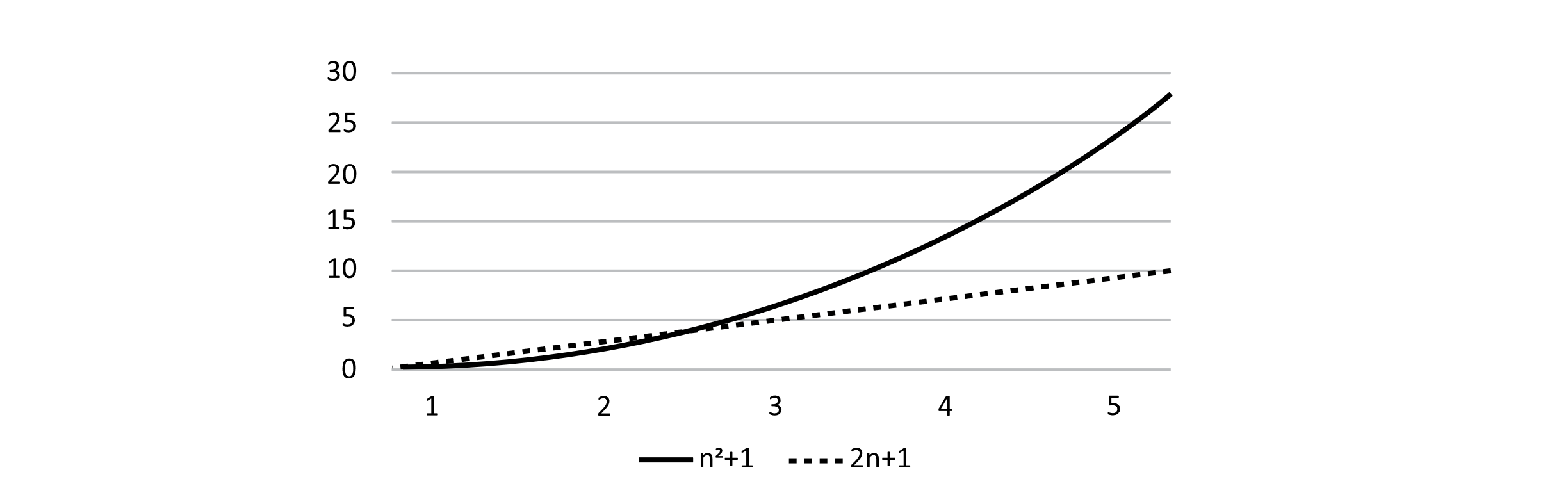
Figure 1.1

Note that when n = 1, your classmate’s algorithm performs fewer operations than our original. However, for all n values that come after 2, the cost of our original algorithm wins outright. Although this does give us some intuition about the performance of algorithms, it would behoove us to define more precise notation before moving forward.

Asymptotic notation gives us a way of describing how the output of a function grows as the inputs become bigger. We will address three different notations as part of this chapter, but the most important is Big-O. Most often stylized with a capital O, this notation enables us to classify cost functions into various well-known sets. Formally, we define Big-O as follows:

While this is a very precise and useful definition, it does warrant some additional explanation:

• O(g(n)) is a set of all functions that satisfy the condition that they are “less than” some constant multiplied by g(n). While it is conventional to say that f(n) = O(g(n)), it is more accurate to read this as “f(n) is a member of O(g(n)).”
• When determining whether a function is a member of O(g(n)), any positive real number may be chosen for c.
• The most important aspect of this notation is that the inequality holds when n is really big. As a result, asserting that it holds for relatively small n values is not necessary. We can choose an n₀. Then for all values greater than it, our inequality must hold.

Through some basic algebra, we can determine that f(n) is O(n), and m(n) is O(n²):

Notably, it is possible to show that f(n) = O(n²). However, it is not true that m(n) = O(n). Showing this has been left as an exercise at the end of the chapter.

Another Example

Someone new to algorithm analysis may start to draw conclusions that cost functions with higher degree polynomials are unequivocally slower (or worse) than those with lower degree polynomials. Consider the following two cost functions and what they look like when n is less than 10:

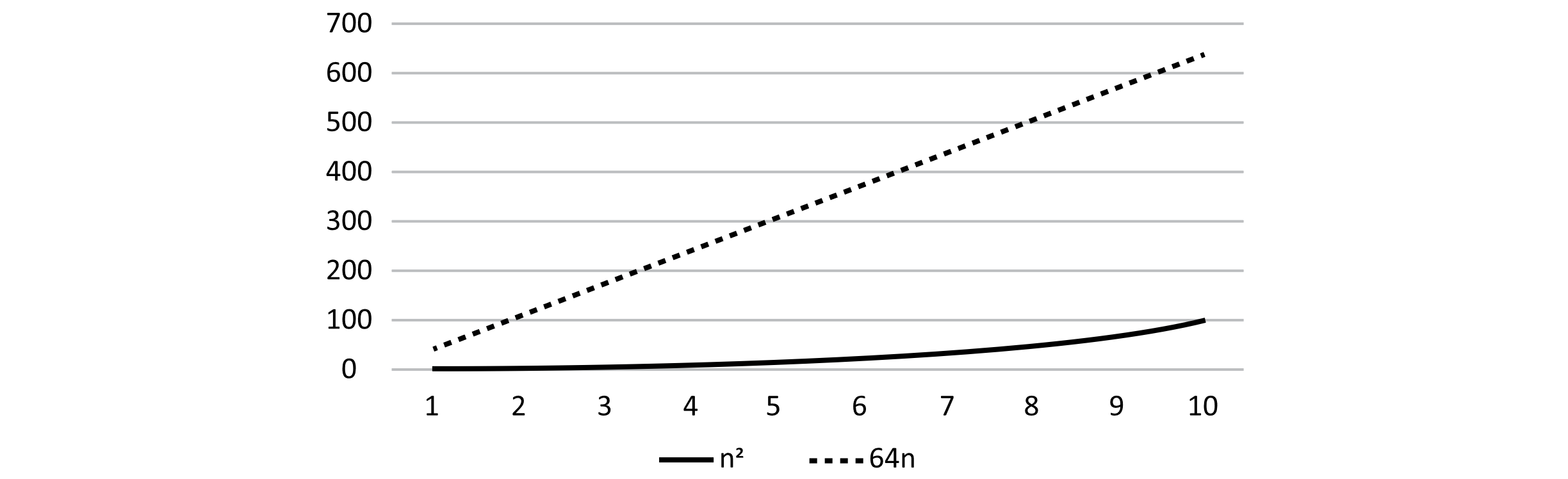
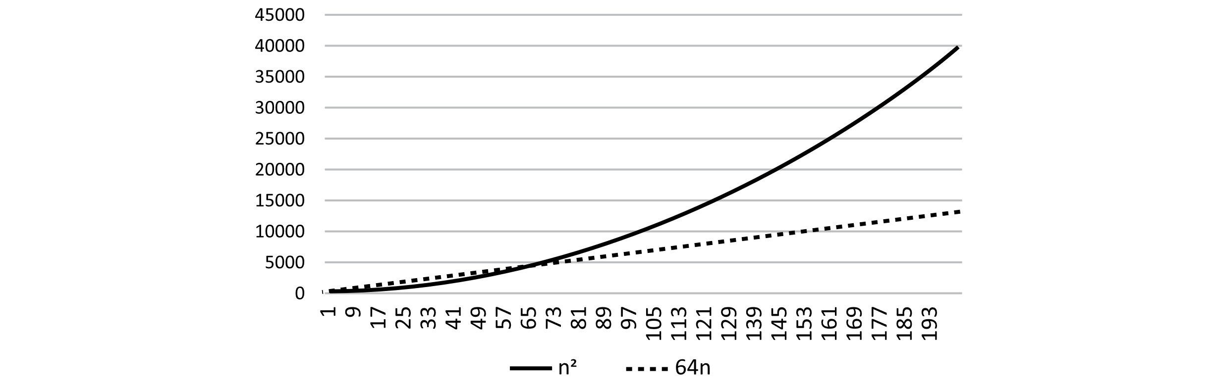
Figure 1.2

As the size of your input (n in this case) gets larger, higher degree terms will always have more influence over the growth of the function than large coefficients on smaller degree terms. It is important though that we do not immediately conclude that the algorithm for function s is inherently better than or more useful than the algorithm for function t. Notice that for small values of n (specifically, those smaller than 64), algorithm t actually outperforms s. There are real-world scenarios where input size is known to be small, and an asymptotically less-than-ideal algorithm may actually be preferred due to other desirable attributes.

Big-O notation captures the asymptotic scaling behavior of an algorithm. This means the resource costs grow as n goes to infinity. It is seen as a measure of the “complexity” of an algorithm. In this text, we may refer to the “time complexity” of an algorithm, which means its Big-O worst-case scaling behavior. If one algorithm runs in O(n) time and the other in O(n²) time, we may say that the O(n) algorithm is an order of magnitude faster than the O(n²) algorithm. The same terms may also be applied to assessments of the space usage of an algorithm.

Other Notations

The remainder of this book (and most books for that matter) typically uses Big-O notation. However, other sources often reference Big-Theta notation and a few also use Big-Omega. While we will not use either of these extensively, you should be familiar with them. Additional notations outside these three do exist but are encountered so infrequently that they need not be addressed here.

Big-Omega Notation

Whereas Big-O notation describes the upper bound on the growth of a function, Big-Omega notation describes the lower bound on growth. If you describe Big-O notation as “some function f will never grow faster than some other function g,” then you could describe Big-Omega as “some function f will never grow more slowly than g.” Herein lies the explanation of why Big-Omega does not see much usage in real-world scenarios. In computer science, upper bounds are typically more useful than lower bounds when considering how an algorithm will perform on a large scale. In other words, if an algorithm performs better than expected, we are pleasantly surprised. If it performs worse, it may take a long time, if ever, to complete. The formal definition of Big-Omega is as follows:

Big-Theta Notation

Big-Theta of a function, stylized as θ(g(n)), has more utility in routine analysis than Big-Omega. Recall that f(n) = 2n+1 is both O(n) and O(n²). This is true because the growth of the function has an upper bound of n as well as n². Although it is possible to reference different functions, it is common to choose the slowest-growing g(n) such that g(n) is an upper bound on function f. We can see that Big-O may not be as precise as we would like, and this can result in some confusion. Therefore, in this book, we will be interested in the smallest g(n) that can serve to bound the algorithm at O(g(n)). As a result of the ambiguity of Big-O, some computer scientists prefer to use Big-Theta. In this notation, we choose to specify both the upper and lower bounds on growth by using a single function g(n). This removes confusion and allows for a more precise description of the growth of a function. The definition of Big-Theta is as follows:

It should be noted that not all algorithms can be described using Big-Theta notation, as it requires that an algorithm be bounded from above and below by the same function.

References

Cormen, Thomas H., Charles E. Leiserson, Ronald L. Rivest, and Clifford Stein. Introduction to Algorithms, 2nd ed. Cambridge, MA: The MIT Press, 2001.