2.2 Introduction

Before learning how to use ultrasound units to assess various anatomical and physiological features, it is essential to learn about the physics behind ultrasound machines. Ultrasound units send ultrasonic waves from a transducer that get reflected from the tissues and are then received by the transducer. The computer processes this information, and images are generated. Transducers utilize the piezoelectric effect to convert the electric pulses to sound waves and vice versa for this image processing. As with any other medical imaging device, ultrasound images are not artifact-free. Multiple different artifacts are associated with ultrasound imaging.

2.3 Ultrasound Machine Components

As shown in Figure 2-1, an ultrasound machine includes the following major components:

• Display—a screen that shows images from the ultrasound scans.
• Keyboard—a key panel for data input and measurement display.
• Central processing unit—a unit that processes signals from and to the transducer.

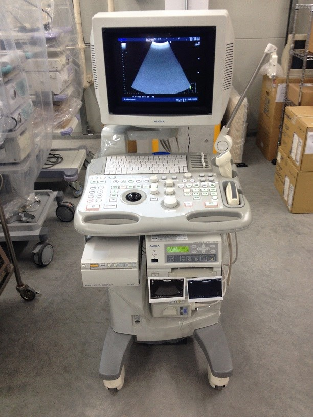
• Pulse controls—dials and controls that are used to change the amplitude, frequency, and duration of ultrasound pulses.
• Transducer—a probe that generates ultrasound waves and detects reflected echoes. It contains piezoelectric materials, which vibrate due to echo pulses from the tissue. The transducer relies on the piezoelectric effect. This piezoelectricity is amplified and transmitted to the display, where it is converted into an image form.
• Amplifier—a unit that increases the size of the electrical pulses coming from the transducer after an echo is received. The amount of amplification is controlled by the gain control knob, which allows the user to adjust the gain to the required depth within the body.
• Storage device (not shown)—a digital device that stores images for later use.
• Printer—a unit that prints images from the displayed data.

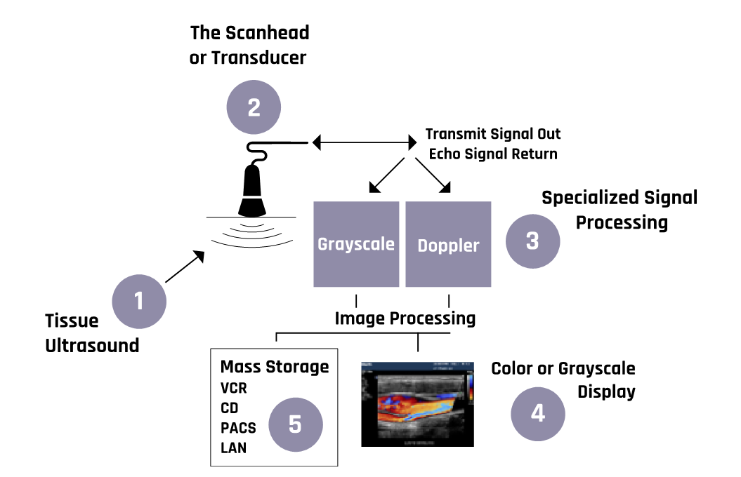
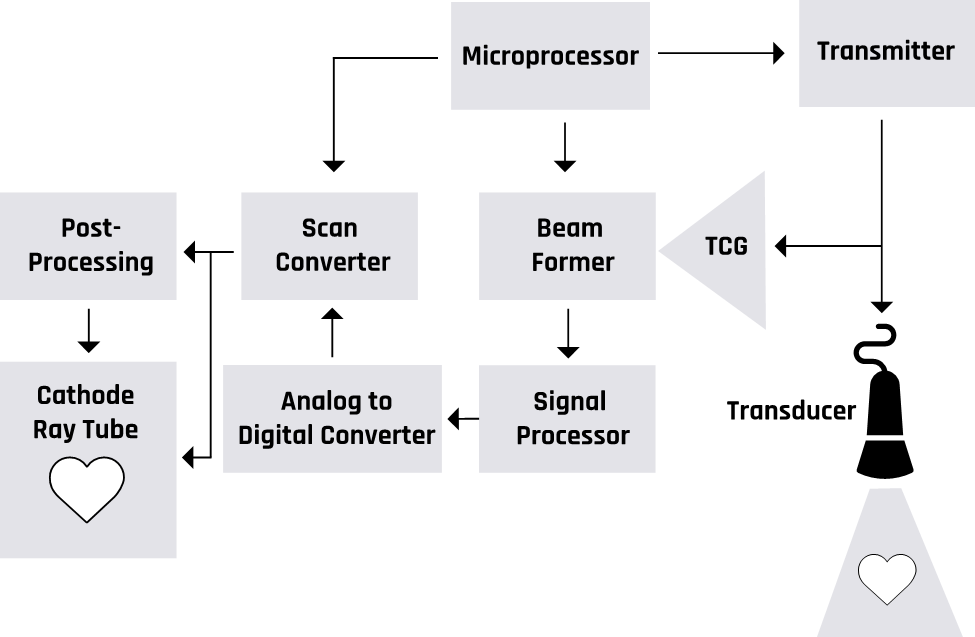
Figure 2-2 shows a generalized schematic of ultrasound machines’ mode of operation.

More details about the operations of the components of the ultrasound machine are discussed in the sections below.

2.4 Piezoelectric Effect

In the 19th century, Pierre and Jacques Curie discovered that some materials generate electric potentials in response to mechanical deformation (material shrinks or expands) or stress (the substance is squeezed or stretched)—a phenomenon called the piezoelectric effect, which is illustrated in Figure 2-3. Conversely, the same materials change their shapes when an electric field is applied.

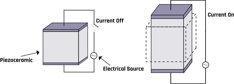
Examples of such materials include silicon oxide, potassium sodium tartrate, barium titanate, and lithium niobate. Bones, tendons, skin, and some man-made polymeric materials can also exhibit the piezoelectric effect. These materials bend in different ways depending on the frequency and their shape, which can result in different vibration modes. The modes are the basis for developing transducers that operate at different frequencies.

2.5 Transducer Characteristics

A typical ultrasound probe with its components is shown in Figure 2-4. The vibration of crystals in an ultrasound machine’s transducer generates ultrasound, and the transducer can detect the echoes and convert them to electrical signals. A transducer is composed of piezoelectric crystals, which respond to pressure to generate an electric current. The alternating current causes the piezoelectric crystals to vibrate at a desired frequency corresponding to ultrasound waves. The produced ultrasound beam is directed into the tissues by moving the transducer and changing the angle of incidence of the ultrasonic beam. Conversely, when an electric current is applied to the crystals, its shape changes with polarity, producing electrical signals from echoes that are processed to generate a display. Hence the crystals act as transmitters (for a short time) and receivers (most of the time).

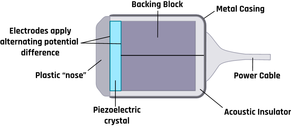
Since the air between the tissue and the transducer inhibits the propagation of the ultrasound beam, a conducting gel is usually applied between them.

2.6 Image Display and Grayscale

Figure 2-5 shows a block diagram of an ultrasound imaging system. Two modes are essential in the formation of an ultrasound image. These are the transmission modes that convert an alternating current into mechanical pressure waves. The backscattered pressure waves are picked up by the receiving mode, which converts them into electrical signals. The ultrasound waves that get fully transmitted through any tissues or structures do not produce echoes and appear dark. For example, all fluids appear echo-free and black on the ultrasound image.

2.7 Pulse-Echo Imaging

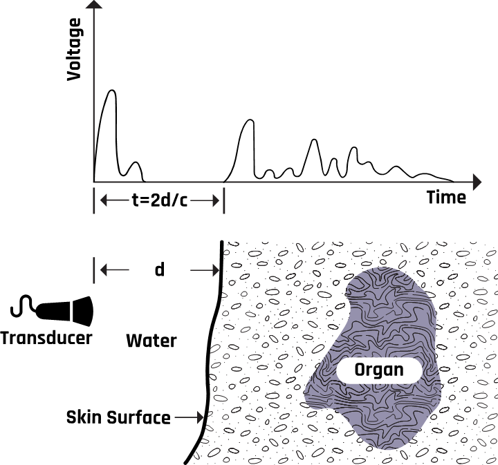
The transducer generates pulses and detects backscattered energy from the tissue boundaries, as shown in Figure 2-6. The length of delay between the transmitted and received pulses is used to determine the depth of the tissue boundary or organ under examination.

These piezoelectric signals from the crystals are amplified and converted into a gray or white color on the ultrasound image via a computer program. The difference in tissue reflectivity allows us to see individual structures. When ultrasound hits a dense object, it is wholly reflected, forming a posterior acoustic shadow (a bright and echogenic image). This is because no ultrasound is transmitted, creating an echo void. The computer can calculate the tissue’s depth by measuring the time between when the wave was sent and when an echo was detected.

2.8 Image Acquisition and Analysis

There are several assumptions about sound waves in ultrasound system operation. These assumptions, when violated, result in the formation of image artifacts, which often make it difficult to distinguish between real and fictitious features in an image. These assumptions are

• the ultrasound beam travels in a straight line with a constant rate of attenuation;
• the ultrasound waves travel directly to a reflecting tissue and back;
• the speed of ultrasound in all soft tissue is exactly 1540 m/s;
• reflections arise only from structures positioned in the beam’s main axis;
• the ultrasound beam is infinitely thin, with all echoes originating from its central axis;
• the strength of a reflection is accurately determined by the characteristics of the tissue creating the reflection; and
• the depth of a reflector is the time taken for sound to travel from the transducer to the reflector and return.

2.9 Artifacts and Errors Associated With Image Acquisition

Artifacts are fictitious portions of images (distortions of the actual anatomy of the tissue). Improper scanning techniques may cause some artifacts, while others result from the physical limitations of the instrument. Such artifacts can be explained using the properties of the ultrasound waves, their propagation through tissue, and the assumptions used in image processing. Typical artifacts include shadowing, beam width, side lobe, reverberation, comet tail, ring down, mirror image, and refraction. They are formed primarily due to multiple echo paths or velocity errors and attenuation errors.

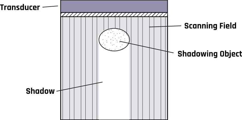
2.9.1 Shadowing Artifact

Highly reflective or attenuating tissues reduce the ultrasound beam intensity inside the tissues, leading to obscured images close to or behind them. This shadowing artifact results from refraction that causes echoes to appear darker, like a shadow, due to the ultrasound beam’s decreased amplitude, intensity, and power.

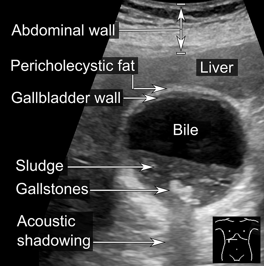
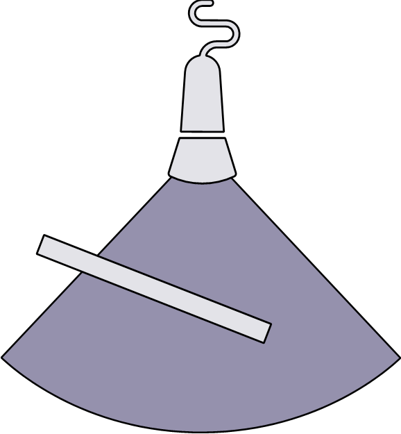
Shadows occur when an ultrasound beam cannot pass through an area deeply due to the presence of a strongly reflecting or attenuating tissue. Figure 2-7 shows acoustic shadowing caused by the stones in the gallbladder. The shadows occur in regions of high acoustic impedance mismatch, such as soft tissue / gas or soft tissue / bone interfaces. These shadowing artifacts prevent visualization of the accurate anatomy on a scan by covering it with an anechoic shadow. This may cause misdiagnosis of the tissue anatomy.

Other causes of shadowing artifacts are improper scanning techniques, improper settings, or poor ultrasound systems.

Some possible ways to reduce these artifacts include taking images from several angles, changing the lateral resolution, or decreasing the frequency to avoid missing information.

2.9.2 Mirror Image Artifact (a.k.a. Ghost Artifact)

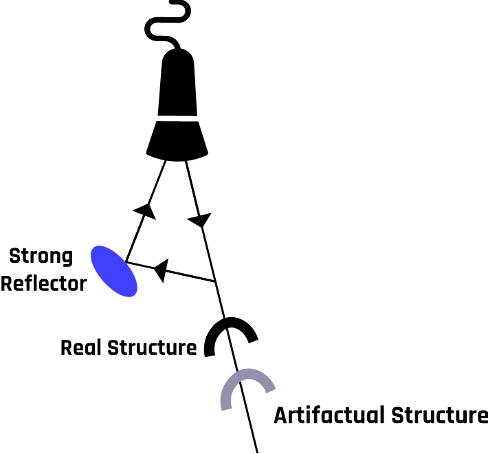
Multiple reflections (reverberation) often occur in regions with high impedance mismatches, such as air/fluid or flesh/bone interfaces. The multiple reflections duplicate a true reflector when the waves from a highly reflective surface are redirected toward a second structure. The redirected waves form a replica of the original structure, which appears on the image as a second structure.

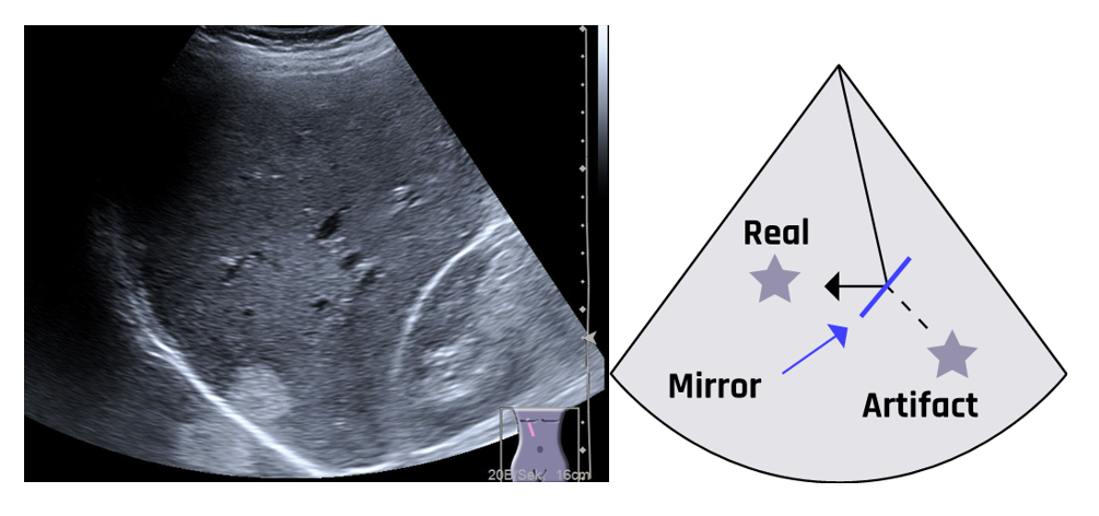
Mirror image artifacts occur in both grayscale and color Doppler imaging. The true reflector and the artifact are equidistant from the mirror plane located between the two, as shown in Figure 2-8. This violates the assumptions that (1) ultrasound waves travel in a straight line and (2) waves travel directly to a reflecting tissue and are reflected directly back to the transducer.

A ghost artifact can develop on a color Doppler image when multiple reflections occur beyond borders. Ghost or mirror image artifacts can be reduced by decreasing the overall gain or changing the beam angle. During diagnosis, mirror images should be clearly separated from actual anatomy, especially in guided needle biopsy, where samples must be taken from a specific location.

Two possible ways by which mirror image artifacts can be formed are illustrated in Figure 2-9a.

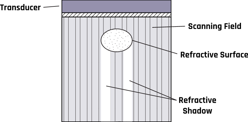
Circular structures such as cysts can cause refraction, which produces shadows on the object’s edge due to a mismatch in acoustic impedance at the boundary or interface. The change in direction (bending) results from the change in the propagation velocity of the ultrasound waves. A schematic of this process is illustrated in Figure 2-9b.

2.9.3 Side Lobe Artifact

Beams generated from the edges of a single-element transducer tend to spread from the primary beam, as shown in Figure 2-10. These lobe beams can be reflected into the primary beam, adding energy to the beam’s main axis. These artifacts violate the assumption that all reflections occur in the path of the beam’s main axis.

This duplication of the true anatomy with false reflection results from strong reflections that return to the transducer. Since the machine assumes all echoes to be coming from a true anatomic structure, incorrect images are displayed together with the correct ones.

A rapidly oscillating ultrasound beam produces multiple side lobe echoes that appear on the display as a curved line equidistant from the transducer. The two most important features that distinguish a side lobe artifact from an anatomical structure are that it is equidistant to the transducer along its length and it passes through anatomical structures.

The side lobe artifact is corrected by imaging the structure in multiple directions. The artifact will not appear in all viewing directions.

2.9.4 Grating Lobe Artifact

While the assumption is that all reflections are in the path of the beam’s main axis, as the beam is projected from the transducer into the tissue, some of the ultrasound waves spread outward, as shown in Figure 2-11. The presence of a strong reflector along the path of the diffracted waves produces echoes that are misinterpreted as being along the beam’s main axis. The grating lobe artifact generally appears weaker than the true reflector. This obscures the actual anatomy with a false reflection.

The artifact is corrected by taking multiple views of the structure under examination. An artifact will not appear in all views.

2.9.5 Multipath Artifact

Multipath artifacts occur when the primary ultrasound beam reflects off anatomy at an angle such that a part of the echo returns to the transducer and at the same time, another echo also reaches the transducer after reflecting off a second boundary.

The echo from the secondary reflector takes a longer path and hence longer time to get back to the transducer. Since ultrasound machines measure the depth based on the time between the transmitted signal and the received echo, the machine will perceive a longer time and depth and position the image on the wrong spot, as shown in Figure 2-12.

In this case, the assumption that the ultrasound beam travels directly to the reflector and back to the transducer is violated. This phenomenon creates what is called a propagation path error. These artifacts give rise to the incorrect axial location of an object due to longer path lengths.

Multipath reflections may form images that appear deeper or misplaced. The problem can be reduced by taking multiple views at different angles.

2.9.6 Curved/Oblique Reflectors

An ultrasound beam incident on a curved or oblique boundary is reflected in various directions. Some of the reflected waves are directed away from the transducer. This reflection is similar to the scattering process. In this case, reflectors do not appear on the image due to longer path lengths and increasing attenuation.

Figure 2-13 illustrates the possible reflections from an oblique surface in various directions. This observation contradicts the assumption that an ultrasound pulse travels directly to a reflecting boundary surface and back to the transducer.

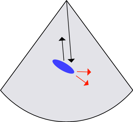
The strength of the echo received by the transducer is less than the expected intensity, which gives false brightness, missing reflections, or an improper location of the anatomic structure. These artifacts are associated with weak, too-bright echoes or improperly located structures. This artifact can be reduced by changing the transducer angle or by using a large footprint.

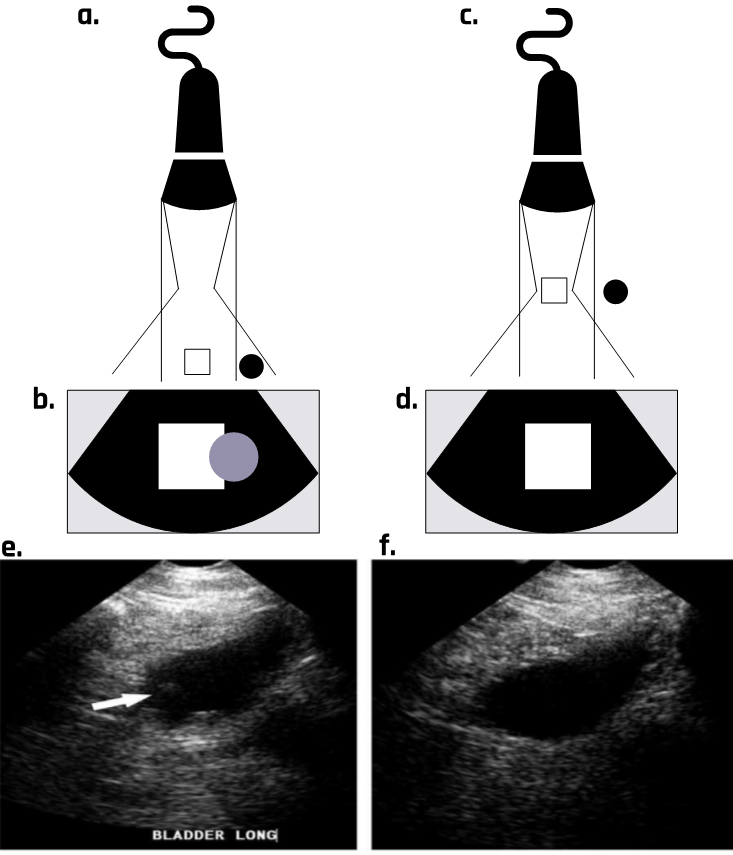
2.9.7 Beam Width Artifact

While it may be convenient to assume that the beam width stays approximately equal to the transducer size, the ultrasound beam actually spreads out as it moves away from the transducer, as Figure 2-14 shows. Due to this divergence, the echoes generated from the edge of the beam appear to be coming from the center of the beam. The artifacts are most apparent when most of the beam travels through the fluid and part of it interacts with adjacent soft tissue, as shown in Figure 2-14.

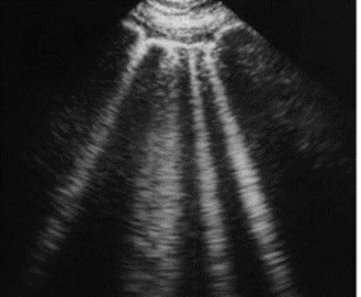
2.9.8 Reverberation Artifact

While the ultrasound machine is based on the assumptions that (1) sound travels in a straight line, (2) all echoes are parallel to the transducer axis, and (3) sound waves travel at 1540 m/s in soft tissue, the ultrasound echoes may be reflected repeatedly between two highly reflective surfaces that are parallel to the primary ultrasound beam. This causes reflections that oscillate between the tissue and the transducer. The artifacts appear on the image as multiple stairways that are equally spaced apart from one another and tend to increase with increasing tissue depth.

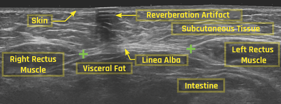
Figure 2-15 shows an image with multiple reflections, indicated by arrows at the top. The first bright line at the top close to the transducer is the only real line image. The other bright images below the actual reflector are artifacts. Another way reverberation artifacts can occur is when the transducer behaves as another reflecting surface such that the returning echoes are rereflected back into the tissue-reflecting structure, resulting in the formation of an identical artifact located at twice the distance from the transducer.

Because of attenuation, each image formed due to subsequent echoes is weaker than the first, as shown in Figure 2-15. The artifact can be prevented by moving the transducer probe at various angles to see an area covered by the artifact.

2.9.9 Comet Tail Artifact

There are various possible causes of comet tail artifacts. These are

• multiple reflections between very closely spaced reflectors;
• small calcifications and the presence of metal objects;
• vibrating small, highly reflective surfaces such as air bubbles; or
• the presence of reflectors in a medium with high velocity.

The artifact typically appears as one or multiple solid bright “tails” parallel to the axis of the primary sound beam, as shown in Figure 2-16. The pattern may differ depending on the size, shape, and composition of the reflecting tissue structure and the scan orientation and distance from the transducer.

This artifact helps diagnose or rule out pneumothorax. If the pneumothorax is present, the air within the pleural space hinders the propagation of ultrasound waves, thereby preventing the formation of comet tail artifacts.

The major problem is that the tails cause significant attenuation such that the beam becomes significantly weak and cannot reach deeper regions of the tissue. These tails prevent the scan from imaging the underside of the reflecting structure. The artifact can be prevented by performing multiple scans at different angles to view the area obscured by the tail.

2.9.10 Propagation Speed Error Artifact

One of the other assumptions of ultrasound machine operation is that the speed of sound in soft tissue is exactly 1540 m/s. However, sometimes the waves may propagate through a medium at a speed other than that of a soft tissue. This produces the correct number of reflectors, which appear at incorrect depths. For speeds greater than 1540 m/s, the depths are underestimated due to the short transmission-reception time of the beam from the transducer to the reflector and back to the transducer. When the sound travels at a speed slower than 1540 m/s, the distances of the reflectors are overestimated.

These artifacts can be reduced by changing the beam’s angle, which may help minimize the difference in propagating speed. Speed error artifacts cannot be prevented entirely. It should be remembered that the artifact causes incorrect placement of the reflectors on the image display.

Care must be taken to identify incorrect placements to avoid misinterpreting the image. This is often achieved by taking images from different angles. If the placement of the reflectors cannot be duplicated at different angles, then the image is an artifact. These speed errors can make the image appear “split” or “cut.” The speed error degrades the quality of an image that relies on resolution, such as the differentiation of lesions and cysts and guided biopsy.

2.9.11 Resolution Artifact

Two assumptions of the ultrasound machine are that echoes come from the main axis of the beam and that sound travels in a straight line. However, very small structures between the beamlines degrade the image detail and produce misleading echoes. The artifact can be prevented by having a higher spatial resolution or line density. Low line density per frame produces poor detail in images. Another cause is excess gain, which tends to create or obscure information and reduce lateral resolution.

The resolution can be corrected by choosing the proper gain or focal zone setting to reduce erroneous echo contrast. An appropriate setting reduces the grainy pattern.

2.9.12 Near Field Clutter

Near field clutter is an artifact that arises from multiple noise sources. Any acoustic noise near the transducer may cause high-amplitude oscillations of the piezoelectric crystals in the transducer. It involves the near field and may hinder the identification of structures that are close to the transducer. These oscillations cause the artifacts to appear and disappear. In general, artifacts change their appearance and appear or disappear depending on the view.

The artifact occurs due to acoustic noise near the transducer, resulting from high-amplitude oscillations of the piezoelectric elements. The appearance of additional echoes from high-amplitude reflections from the transducer in the near field can overshadow the weaker echoes from true anatomic structures. Nevertheless, when viewed from multiple angles, the real tissue structures will remain constant, while the artifacts will appear and disappear as the scan angle changes.

2.9.13 Ring Down Artifact

This artifact is caused by small gas bubbles, which produce reflections after the transducer receives the initial reflection. The transducer sees the echoes as though they are coming from structures in the deeper part of the tissue. The pocket of fluid and air continuously resonates, reflecting ultrasound and creating a hyperechoic region. This process commonly occurs in regions with air bubbles and water.

The artifact generally appears as very bright and continuous parallel bands extending to the image’s bottom. Its brightness makes it hard to view the region beneath it. The effect can be reduced by moving the scanning beam at different angles.

2.9.14 Enhancement Artifact

This artifact is the opposite of the shadowing effect due to low attenuation. It is common in fluid-filled structures such as the gallbladder, the urinary bladder, or cysts due to excessive brightness. The primary causes are improper ultrasound settings and scanning techniques.

2.9.15 Focal Enhancement and Banding Artifact

Focal enhancement is formed due to attenuation effects, improper ultrasound settings, and improper brightness, which cause the sound waves to weaken as they propagate in the medium. This is because the amplitude decreases.

2.9.16 Refraction Artifact

The change in the propagation speed of ultrasound due to differences in impedance causes the transmitted beam to change its direction after passing through the boundary. When the beam moves from one medium to another with a higher (or lower) impedance, the transmitted beam is refracted toward (or away from) the normal at the point of incidence.

This phenomenon occurs when a beam hits the interface obliquely, creating separate beams with different propagating speeds, contrary to the assumption that sound travels in a straight path. This can create a duplication of the anatomic features. For example, refraction may cause a single feature to appear as a double feature.

2.9.17 Slice Thickness Artifact

A propagating artifact appears when the beam dimension is far greater than the reflector size. Another possible cause is improper elevation resolution. The artifact “creates” debris that appears in cyst images, which can lead to false diagnoses. This is because the image plane is neither extremely thin nor uniform, as assumed. Using tissue harmonic imaging and thinner transducer arrays would reduce the problem.

2.10 Transducer Arrays

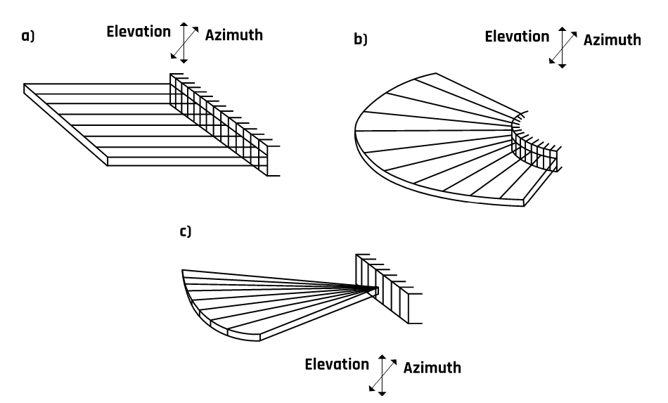
Transducers are available in various shapes and sizes depending on users’ needs. As discussed earlier, a transducer consists of piezoelectric crystals—not one crystal but an array of multiple crystal elements. The various arrays and transducers are discussed below, and their schematics are shown in Figure 2-17.

2.10.1 Linear Sequential Arrays

Modern linear ultrasound transducers contain 256 to 512 elements. Their advantage is high sensitivity when directed perpendicular to the surface under examination. However, the beam cannot be steered, which limits the field of view.

2.10.2 Curvilinear or Convex Arrays

The arrays are similar to those in the linear array but are curved, which gives them the advantage of scanning a wider field of view than linear arrays.

2.10.3 Linear Phased Arrays

Phased arrays have much smaller elements than those in a linear array. Typically, they contain 128 elements to transmit and receive each data line. Linear phased arrays are typically used for viewing restricted acoustic windows.

2.11 Image Display Modes

Ultrasound images are generated when the transducer transforms the reflected wave or echo from the mechanical energy of vibration into an electrical signal that is converted into an image on the display. The image can be displayed in any of the following three modes: (1) amplitude (A) mode, (2) brightness (B) mode, or (3) motion (M) mode. These are discussed in detail in the sections below.

2.11.1 A-Mode Display

The A-mode is the first form of image display. The depth (reflector-time relationship) is represented on the horizontal axis, and amplitude is displayed on the vertical axis. The A-mode measures the reflectivity at different depths under the transducer. It is commonly used for examining the eyes, the liver, and the brain. Low frequencies of 2–5 MHz are used for abdominal, cardiac, and brain scanning. Organs such as the eyes and peripheral blood vessels use a 5–15 MHz frequency.

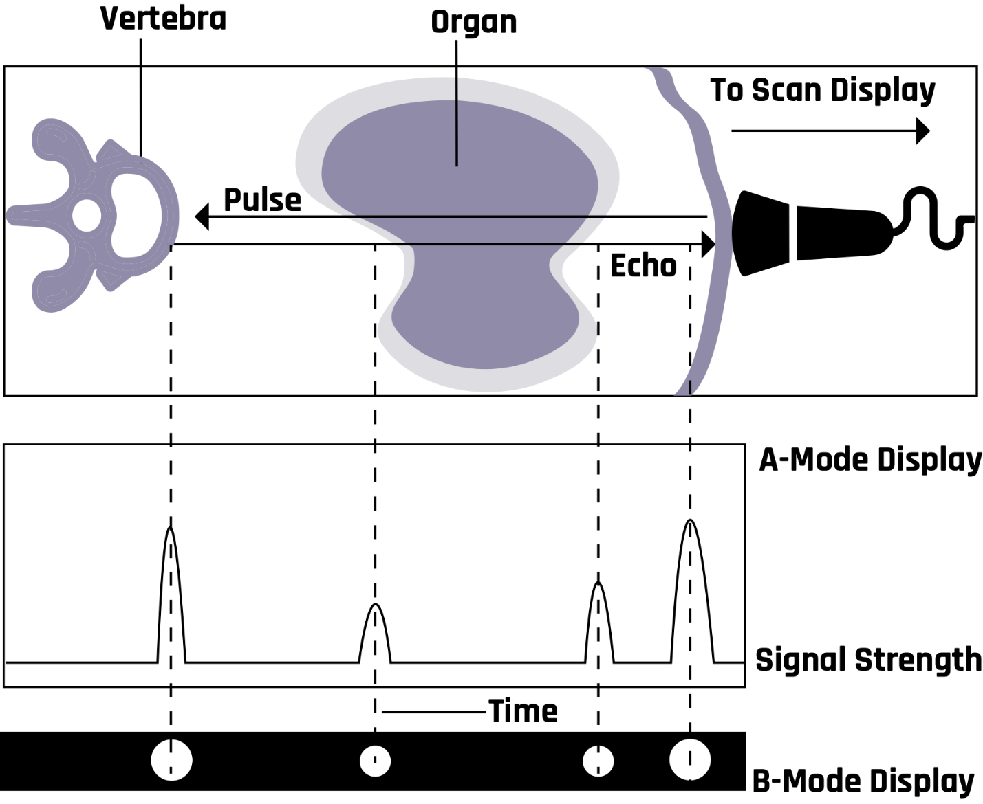
2.11.2 B-Mode Display

In the B-mode, the echoes are represented by bright dots. A shade of gray is assigned to each echo. The brightness of the dots indicates the strength of the echoes. The position of a dot on the screen represents the reflector distance and is determined by the transducer-reflector time relationship. Many diagnoses are made in the B-mode (in black and white) with a relatively simple probe and protocol. It finds use in the study of both stationary and moving structures. The B-mode is an electronic conversion of the A-mode and A-line information into brightness-modulated dots on the display screen, as illustrated in Figure 2-18.

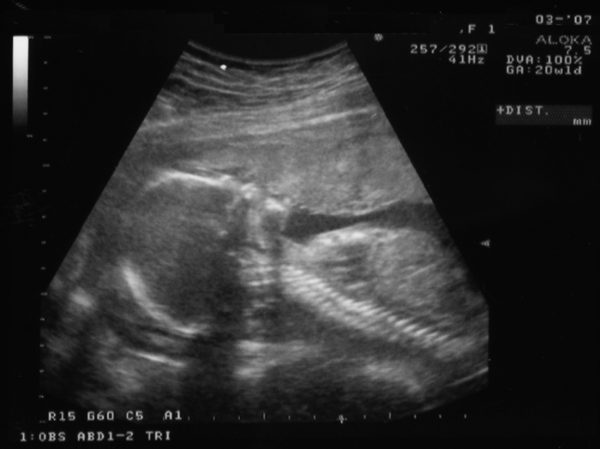
The B-mode display can be used for the M-mode and 2D grayscale imaging. Modern B-mode ultrasound uses both the fundamental and the second harmonic frequencies. Harmonic imaging is most useful in patients with thick and complicated body wall structures. Figure 2-19 shows anatomical structures in the B-mode.

The B-mode is also used for early intima-media thickness analysis of the carotid arteries (located in the neck) to determine the potential for lethal cardiac events. Abnormal thickening of the arterial walls of the carotid arteries is an early indicator of vascular disease throughout the body. The thicker the arterial wall, the greater the risk of heart attack or stroke.

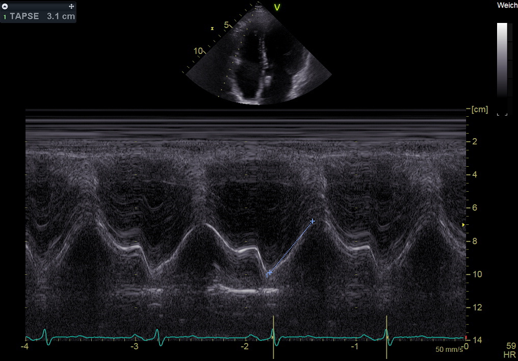
2.11.3 M-Mode Display

In the M-mode, the motion of an object points along the transducer axis and is revealed by a bright trace moving up and down across the image. This display is commonly used to evaluate the morphology, movement, and velocity of cardiac valves and walls.

Imaging the pattern of moving cardiac structures over time constitutes M-mode echocardiography, as Figure 2-20 shows.

2.12 Doppler, Color Flow, Color Power, and Duplex Ultrasound

Doppler imaging is based on the Doppler effect, which shows the relationship between velocity and frequency shift. This imaging system is mainly used to measure blood flow velocity to determine any narrowing of the arteries and assess the risk of stroke occurrence.

In the sonographic application of the Doppler effect, a typical moving source would be flowing blood, and a typical receiver would be a stationary transducer. When the source is moving away, the detected frequency is lower. Conversely, a source moving closer to the receiver would have a higher detected frequency.

For a stationary source (transducer) and a receiver (target) moving with velocity (v) at an angle (θ) relative to the direction of the incident wave of frequency (f_s) from the transducer, the Doppler frequency is given by

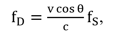
where c is the speed of sound in the tissue, which is 1540 m/s.

The transducer transmits and receives sound waves in the form of sinusoidal signal waves. The magnitude of the Doppler shift is related to the velocity of the blood cells or moving tissue, and the polarity of the shift reflects the direction of blood flow. The blood flowing toward the transducer is positive, and the blood flowing away from the transducer is negative.

The Doppler shift (Δf) is directly proportional to the velocity (v) of the blood cells, the transducer frequency (f_s), and the cosine of the angle of incidence (θ) and is inversely proportional to the velocity of sound in tissue (c = 1540 m/s). In cardiac applications, the angle of incidence in the Doppler equation is assumed to be 0 or 180 degrees.

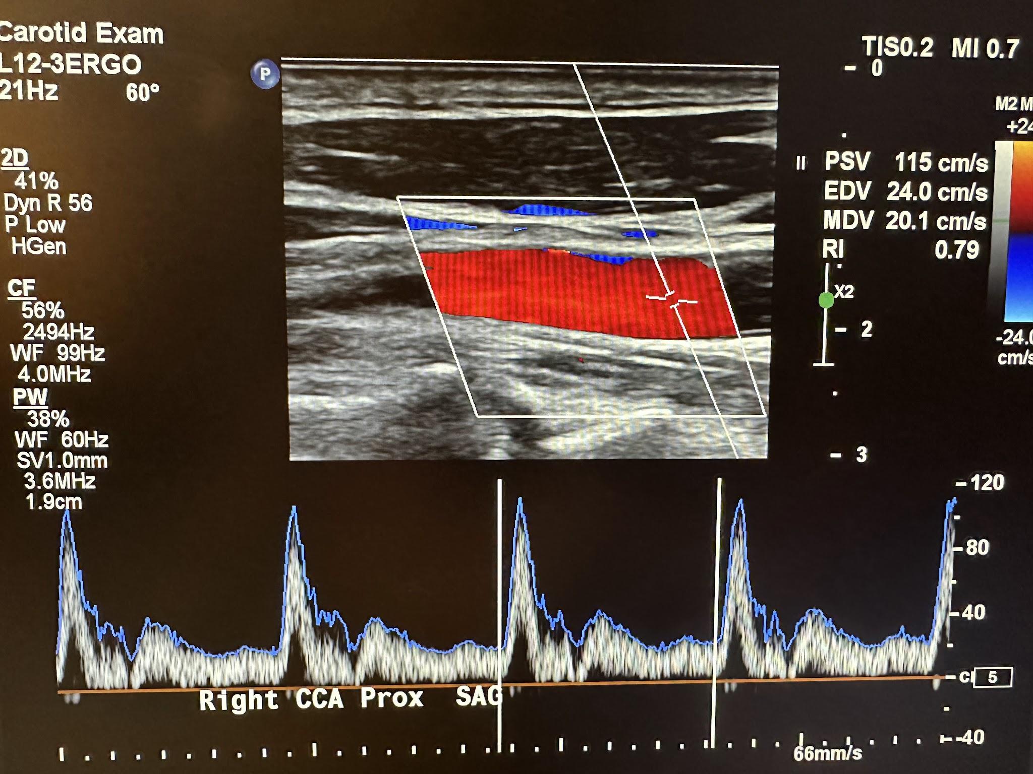
Three modalities are currently used in Doppler echocardiography, and these are pulsed wave (PW) Doppler, continuous wave (CW) Doppler, and color flow (CF) Doppler imaging. Color flow imaging evaluates the Doppler flow information for its direction toward or away from the transducer based on the color display. A commonly used acronym for remembering the color and direction is BART—blue away, red toward. The PW Doppler does not continuously transmit and receive the ultrasound pulse. Multiple crystals in the transducer are excited in a quick burst, producing ultrasound waves. This transmission burst is then followed by a “listening” period during which the crystals detect the reflected signals. Signals from more superficial structures are received sooner than those from deeper structures with more extended “listening” periods. This feature allows signals only from specific depths to be processed, thereby controlling sample size and range resolution. Therefore, two vessels located above each other can be evaluated separately, and vessels can also be followed as their courses change. The PW Doppler wave is site-specific and can only measure low-flow velocities—it cannot correctly measure high velocities (above 1.5–1.7 m/s). The CW Doppler uses two piezoelectric crystals, one to emit ultrasound continuously and the other to receive the reflected waves continuously. This results in a fixed sample size and no range resolution or ability to place the sample volume at a specific depth. It also cannot create anatomic images. It is used for precise settings such as very high peak systolic velocities.¹ The CW Doppler measures very high blood flow velocities, and the color flow CF Doppler is a PW Doppler with multiple gates that allow it to measure the flow velocity through the heart on the two-dimensional echocardiographic image. Physicians often use Doppler imaging to detect blockages to the blood flow (due to clots), constriction of vessels or tumors, and congenital vascular malformations. Figure 2-21 shows an ultrasound image of the right common carotid artery and the corresponding Doppler waveform.

Duplex ultrasonography combines physiologic information based on Doppler shift frequencies with anatomic information from real-time, high-resolution B-mode imaging.

2.13 Blood Flow Dynamics

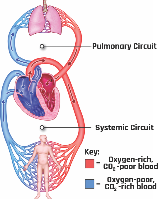
Understanding blood flow dynamics is important in the study of vascular disease development, such as atherosclerosis, thrombosis, or aneurysms. The circulation system transports nutrients and waste around the body (delivering oxygen and nutrients to the cells and removing cellular wastes and carbon dioxide). Its other function is to maintain a constant temperature and potential or power of hydrogen (pH) in all organs of the body. The circulation system comprises the heart (the pump that drives the blood to all body tissues), blood vessels (delivery routes), and blood (the medium that transports the food and the waste materials). The blood flows continuously through two separate loops that originate and terminate at the heart: the pulmonary circulation and systemic circulation loops, as shown in Figure 2-22. Pulmonary circulation carries blood between the heart and lungs, and systemic circulation carries blood between the heart and the body’s organs and tissues. At any time, about 84% of the entire blood volume is in systemic circulation, 7% is in the heart, and 9% is in the pulmonary vessels.

Under normal conditions, the average resting heart rate of an adult between the ages of 18 and 80 is about 75 beats/min, with a stroke volume of 70 mL/beat (cardiac output of 5.25 L/min). For vigorous-intensity physical activity, the heart rate can increase to as high as 200 beats/min, with a stroke volume of up to 150 mL/beat (cardiac output of about 25 L/min).^[1] The arteries respond to varying pressure conditions by dilating or shrinking to accommodate the hemodynamic demands.

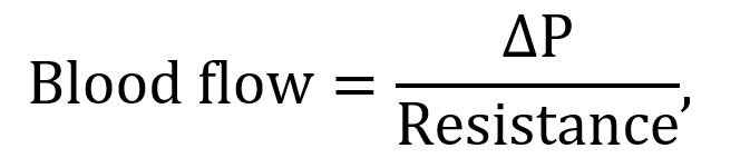
The presence of a pressure gradient between the aorta and the veins ensures the blood keeps moving to the peripherals. In mathematical form, the volume per unit time (Q) can be expressed using Dacy’s law: Q = ΔP/R, where ΔP is the pressure differential and R is the resistance. Figure 2-23 shows the systemic blood pressure throughout different paths of the body.

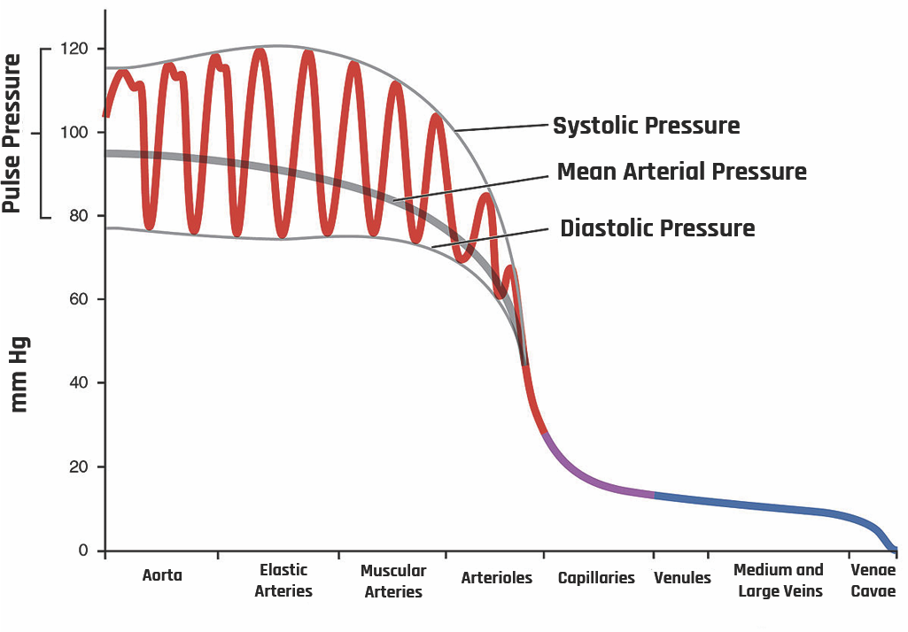
As the heart pumps the blood, the pressure varies between systolic pressure (pressure peak after ventricular systole) and diastolic pressure (pressure drop during ventricular diastole). In the aorta, the systolic average pressure is about 120 mm of Hg, while the diastolic average pressure is about 80 mm of Hg.

The velocity of the flow is mainly determined by three critical variables: radius (r), vessel length (λ), and viscosity (η), which are related to one another by Poiseuille’s equation:

where ΔP is the pressure differential and resistance is given by

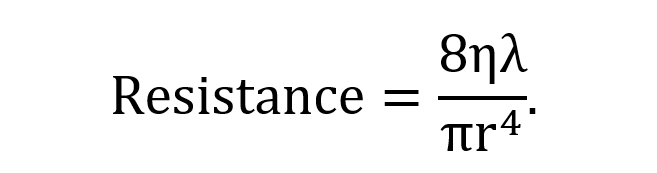
This shows that since the radius changes with vasoconstriction and vasodilation, the effect will be a dramatic change in the resistance and flow of blood.

The blood flow through straight, long, and smooth vessels is almost linear, with each layer of blood remaining the same distance from the walls of the vessels. These different layers flow at different velocities. Speed is dependent on both the axial distance and pressure. At high pressure, the velocity is high, whereas at low pressure, the velocity is low. This leads to a decrease in pressure and velocity from the heart to peripheral circulation.

Due to the difference in systolic and diastolic pressures, pulse pressure is generated during systole. A pulsatile blood flow is created down the pressure gradient into systemic circulation. The pulse pressure is ~ 40 mm of Hg, the difference between systolic and diastolic pressures.

2.13.1 Laminar Versus Turbulent Flow

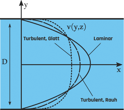
In a laminar flow, the motion of the fluid is very orderly, with all particles moving in straight lines parallel to the walls of the tube, as shown on the left of Figure 2-24. The velocity profile across the tube is parabolic, with the fluid’s highest velocity at the tube’s center, as shown in Figure 2-25. The parabolic profile arises because the fluid molecules touching the walls experience more resistance than those at the center.

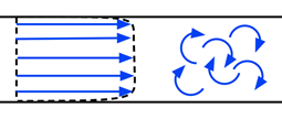
When the velocity of the blood becomes too high as it passes through a constricted vessel or a rough surface, the flow may become irregular, resulting in random fluctuations in position and time, leading to turbulent flow.

The tendency for turbulent flow is measured using the Reynolds number, which depends on the velocity of the flow, the diameter of the vessel, and the density of the blood:

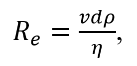
where ν is the average blood flow velocity (in cm/s), d is the vessel diameter (in cm), ρ is density, and η is the viscosity of the blood. In these units, turbulence occurs when R_e > 200, resulting in the formation of eddies. Turbulence can occur in regions of stenosis with increased flow velocity. This type of flow is not common in healthy vessels.

2.13.2 Renal Resistive Index

The renal arterial resistive index (RI) is measured as

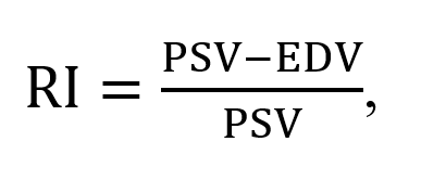
where PSV and EDV represent the peak systolic velocity and end-diastolic velocity, respectively.

The RI index is used as an indicator for detecting and managing renal artery stenosis, evaluating risk in chronic kidney disease, compiling differential diagnoses in acute and chronic obstructive renal disease, and predicting renal and global outcomes in critically ill patients.

Recent studies have shown that an increased RI reflects changes in intrarenal perfusion and systemic hemodynamics and the presence of subclinical atherosclerosis and, therefore, may provide valuable prognostic information for patients with primary hypertension.^[2]