6 Musculoskeletal Sonography

6.2 Introduction

Ultrasound can be used to evaluate different anatomic MSK structures for diagnostic and therapeutic purposes. In particular, protocols have been developed to evaluate different joint structures of the upper and lower extremities. A complete MSK ultrasound of an extremity incorporates real-time scanning of a specific joint, including muscles, tendons, ligaments, or other structures and any abnormalities. A limited MSK ultrasound is a focused evaluation of a specific anatomic structure, such as a tendon or muscle injury. To develop competence in MSK evaluation, being familiar with anatomy, function, and pathology is imperative. This chapter will introduce fundamental structures we find in routine MSK sonography.^[1]

6.3 Performing a Diagnostic Exam

In general, transverse and longitudinal planes (also called sagittal planes) should be obtained of all key anatomic structures and pathologies when performing a diagnostic evaluation. It is always important to know your orientation when visualizing the images. Transducers usually have an indicator on one side at the end of the probe, such as a light, knob, or notch corresponding to the right side of the screen’s image. If you are unsure, just touch one edge of the probe with your finger, and look at the screen to see if you are on the right or left side before imaging. During the evaluation, compare static images, dynamic images, Doppler evaluation, and possible contralateral evaluation. Also, document any masses or fluid collections, such as bursal distension, by indicating the location, size, shape, echotexture, compressibility, and presence or absence of flow with Doppler.^[2]

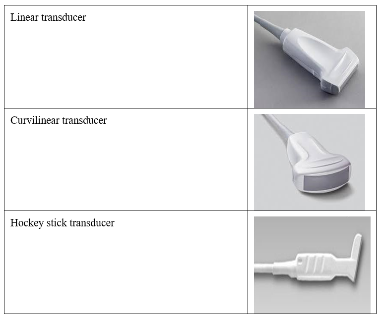
Image optimization is obtained by selecting the proper transducer with appropriate frequencies. In general, a high-frequency linear transducer (10 MHz or higher) will be the appropriate selection for the evaluation of most joints. However, sometimes a curvilinear transducer gives better imaging in larger joints and in the evaluation of most adult hips, which usually require deeper penetration for visualization. Another exception would be the evaluation of superficial detailed structures such as the pulley system of the digits in the hand. A hockey stick transducer (>10 MHz) would be more appropriate for better resolution. Figure 6-1 shows some commonly used transducers in musculoskeletal ultrasound assessment. When evaluating a joint, it is helpful to start by directing your angle of insonation to the bony cortex, which is usually the most distal and hyperechoic structure, to avoid anisotropy.^[3]

6.4 Identifying Abnormal Structures

The normal sonographic appearance of MSK structures often has characteristic ultrasound images that are best visualized in the longitudinal plane. For example, tendons usually appear as a hyperechoic fibrillar echotexture. Ligaments are similar but more compact and connect two osseous structures. Muscle tissue appears more hypoechoic with septations, a pennate (featherlike) appearance in the longitudinal plane, and a starry-night appearance in the transverse plane with dynamic maneuvers. Bone is usually very hyperechoic. It creates a significant acoustic impedance mismatch and therefore is very reflective and appears bright white (hyperechoic) on the image. Adipose tissue and cartilage tend to be hypoechoic. Nerves tend to have both a hypoechoic and hyperechoic honeycomb appearance. The location and function of the structures are always helpful when determining normal anatomy and pathology.

Injuries, inflammation, or infections are divided into acute and chronic and can affect any musculoskeletal structure. Acutely, the sonographic structures tend to be hyperechoic, with possible hypertrophy, hypervascularity, fluid, and disruption of fibers in structures such as tendons. Chronic sonographic images tend to be more hypoechoic, with possible atrophy, scarring, and areas of calcification. Bone abnormalities can also be seen in acute and chronic processes. The normal bone cortex is smooth, uniform, and hyperechoic. A bone fracture can be visualized as a discontinuity of the bone cortex and disruption of the cartilage. Arthritis can have characteristic bone images such as crystal deposits on the cartilage surface in gout and synovial hypertrophy with bone erosions in rheumatoid arthritis.

Sonographic artifacts are not uncommon with MSK ultrasound, some of which have been discussed in earlier chapters. It is vital that the sound beam is perpendicular to the anatomic structure being visualized, or anisotropy can be encountered and give false information. To correct for anisotropy, performing a heel-to-toe maneuver on the long axis and toggling the transducer on the short axis are often helpful to finely tune the ultrasound image.

6.5 Shoulder Sonography

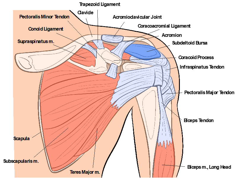
Figure 6-2 shows the anterior view of the shoulder anatomy. The shoulder is one of the most accessible joints to perform a comprehensive ultrasound evaluation. An ultrasound evaluation can be as reliable as an MRI for a rotator cuff tear. A complete shoulder evaluation should include the rotator cuff’s tendons and muscles, including the subscapularis, supraspinatus, infraspinatus, and teres minor. Also, examine the biceps brachii (with dynamic maneuvers, if indicated for subluxation, dislocation, or impingement), the acromioclavicular joint, the suprascapular nerve (in the suprascapular notch and the spinoglenoid notch), and the posterior glenohumeral joint.^[4] Evaluating each anatomic structure in the transverse and longitudinal planes is essential.

For examination of the patient’s shoulder, developing an approach that allows for the best visualization with dynamic maneuvers is helpful. One approach would be to start by standing in front of the seated patient with their arm at their side, the elbow at 90 degrees flexion, the forearm in supination, and the ultrasound machine on one side of the patient for exam visualization.

The long-head biceps tendon is the first structure to be evaluated, and it works as a good reference point for the anterior shoulder evaluation. The origin of the long-head biceps is the supraglenoid tubercle of the scapula, and the insertion is the radial tuberosity and bicipital aponeurosis. It is innervated by the musculocutaneous nerve. Its action is flexion and supination of the forearm at the elbow joint and flexion of the arm at the shoulder joint. First, look at the transverse position within the bicipital groove of the humeral head with a linear transducer.

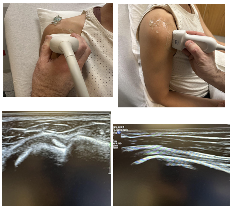
The biceps tendon should have a bright, dense, ovoid, and bristle-like appearance. It should be assessed from proximal to distal in the transverse and longitudinal planes, as shown in Figure 6-3. It is essential to evaluate the most proximal area where the biceps tendon courses over the humeral head because this is a common site for pathology. Also, fluid distension within the bicipital tendon sheath often indicates shoulder pathology, since part of it communicates with the shoulder joint. Continue the evaluation distally until the fibrous-appearing band of the pectoralis major inserted into the proximal humerus is visualized. This is sometimes where a bicipital tendon tear can be found separated from the muscle after an injury. Dynamic maneuvers, both active and passive, can be very helpful in the evaluation.

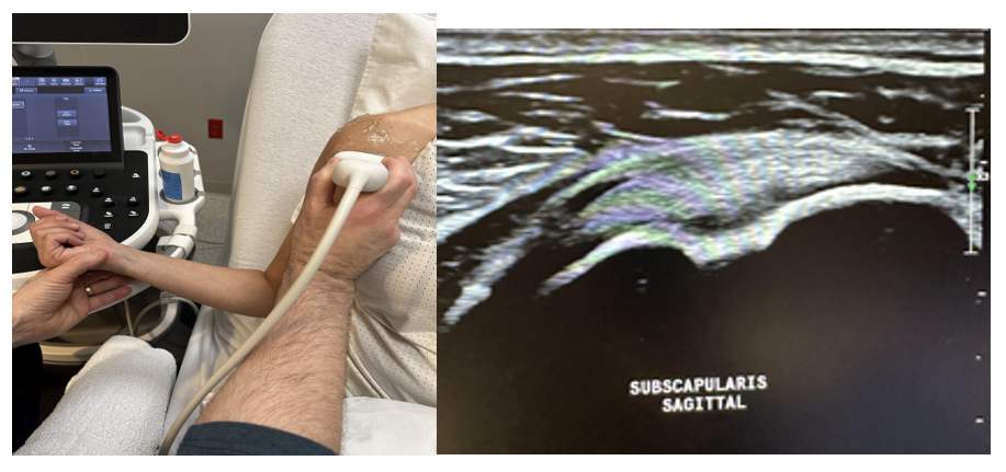
After looking at the bicipital tendon/muscle, return to the point of reference within the bicipital groove of the humerus in the transverse plane. Next, evaluate the subscapularis, which originates at the subscapular fossa and inserts into the lesser tubercle of the humerus. It is innervated by the upper superior and lower inferior subscapular nerves, and the action is for internal rotation of the humeral head. It prevents anterior displacement of the humerus. First, start by moving the transducer medially to the lesser tuberosity to evaluate the rotator interval, which is the space between the anterior margin of the supraspinatus tendon and the superior margin of the subscapularis tendon. The subscapularis tendon/muscle is evaluated by a passive range of motion with external rotation, as shown in Figure 6-4. This brings the subscapularis into the longitudinal (sagittal) plane as it rotates over the humerus. During this dynamic maneuver, also evaluate for coracoid impingement. A limited view of the anterior glenohumeral joint can also be evaluated in this position. The probe is then rotated 90 degrees clockwise in the transverse plane. In this view, the subscapularis will have a characteristic vertical hypoechoic segmented appearance secondary to the musculoskeletal junction, which is usually normal anatomy and not a tear. The evaluation should again include any evidence of effusion, synovial hypertrophy, or tearing.^[5],^[6]

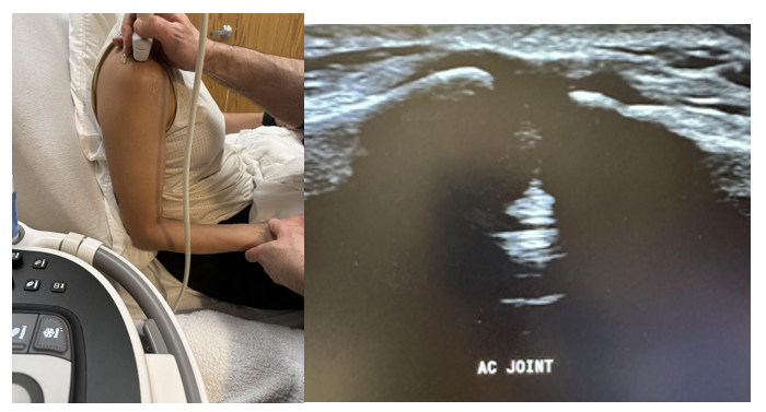
The next anatomic structure to evaluate in the anterior position of the patient is the acromioclavicular (AC) joint, shown in Figure 6-5. The most straightforward approach is to palpate the AC joint and place the linear transducer on top of it in the transverse plane. Evaluate for widening, such as in a tear or effusion, which is sometimes indicative of rotator cuff pathology.

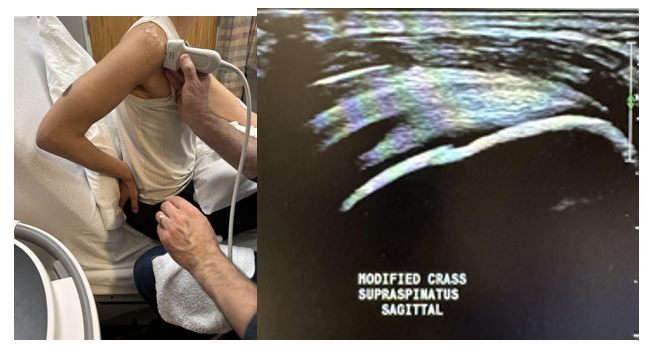
The next rotator cuff to be evaluated is the supraspinatus, which originates in the supraspinatus fossa and is inserted on the superior facet of the greater tubercle of the humerus. Innervation is by the suprascapular nerve; its action is the abduction of the arm and stabilization of the glenohumeral joint. The best position for the patient to be in is called the modified crass position. In this position (which involves extension, adduction, and internal rotation), the patient is sitting upright with the palm of their hand on the ipsilateral hip and the elbow flexed and pointed posteriorly. This brings the supraspinatus out from under the cover of the acromion. Over 90% of rotator cuff injuries involve the supraspinatus.^[7],^[8] First, evaluate the supraspinatus tendon in the longitudinal plane, as shown in Figure 6-6. This image is the most essential view and should have a bird’s beak appearance. Next, include the transverse plane view. Evaluate the bony cortex, hyaline cartilage, supraspinatus tendon/muscle, peribursal fat, and the subacromial bursa. Pooling of fluid within the subacromial bursa or restrictive motion of the supraspinatus tendon could indicate subacromial impingement.^[9]

It is vital to evaluate the tears of the supraspinatus with the correct description. First, determine if it is a full-thickness tear extending from the articular to the bursal surface or a partial-thickness tear. Partial-thickness tears involve the articular or bursal surface or are localized within the tendon, not extending to either surface. This is called an intrasubstance tear. When evaluating the diameter of the tear, measure along the long and short axis.

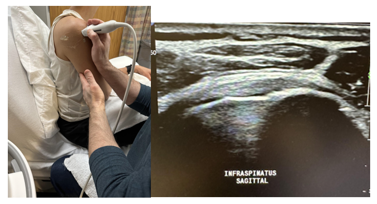
Posterior cuff imaging is evaluated next by facing the posterior shoulder, palpating the scapular spine, and placing the transducer below it in an oblique axial plane angled superiorly toward the humeral head. A curvilinear probe is sometimes needed for better penetration, since the posterior shoulder is a deeper structure. The infraspinatus and teres minor tendons are first evaluated in the longitudinal plane from the scapular fossa’s origin to the humerus’s greater tuberosity, as shown in Figure 6-7. The origin of the infraspinatus is the infraspinatus fossa of the scapula, and the insertion is on the middle facet of the greater tuberosity of the humerus. The suprascapular nerve innervates it, and its action is for external rotation and abduction of the arm at the shoulder joint with stabilization of the shoulder joint. The teres minor originates on the lateral border of the scapula and inserts onto the inferior facet of the greater tuberosity of the humerus. It is innervated by the axillary nerve and functions similarly to the infraspinatus.

Next, evaluate the suprascapular nerve in the suprascapular notch and the spinoglenoid notch. Sometimes, turning on the Doppler to better visualize the suprascapular artery is helpful, and right next to it is the suprascapular nerve.

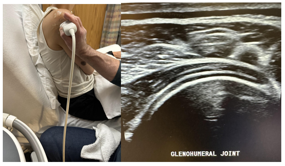
Finally, evaluate the posterior glenohumeral joint, as shown in Figure 6-8. Look for joint effusion, cortical irregularities, and osteophytes, and evaluate the posterior labrum for cysts or tears. Also, this is a good approach for intra-articular glenohumeral joint injections using a posterior approach. This completes the shoulder evaluation.

6.6 Elbow Sonography

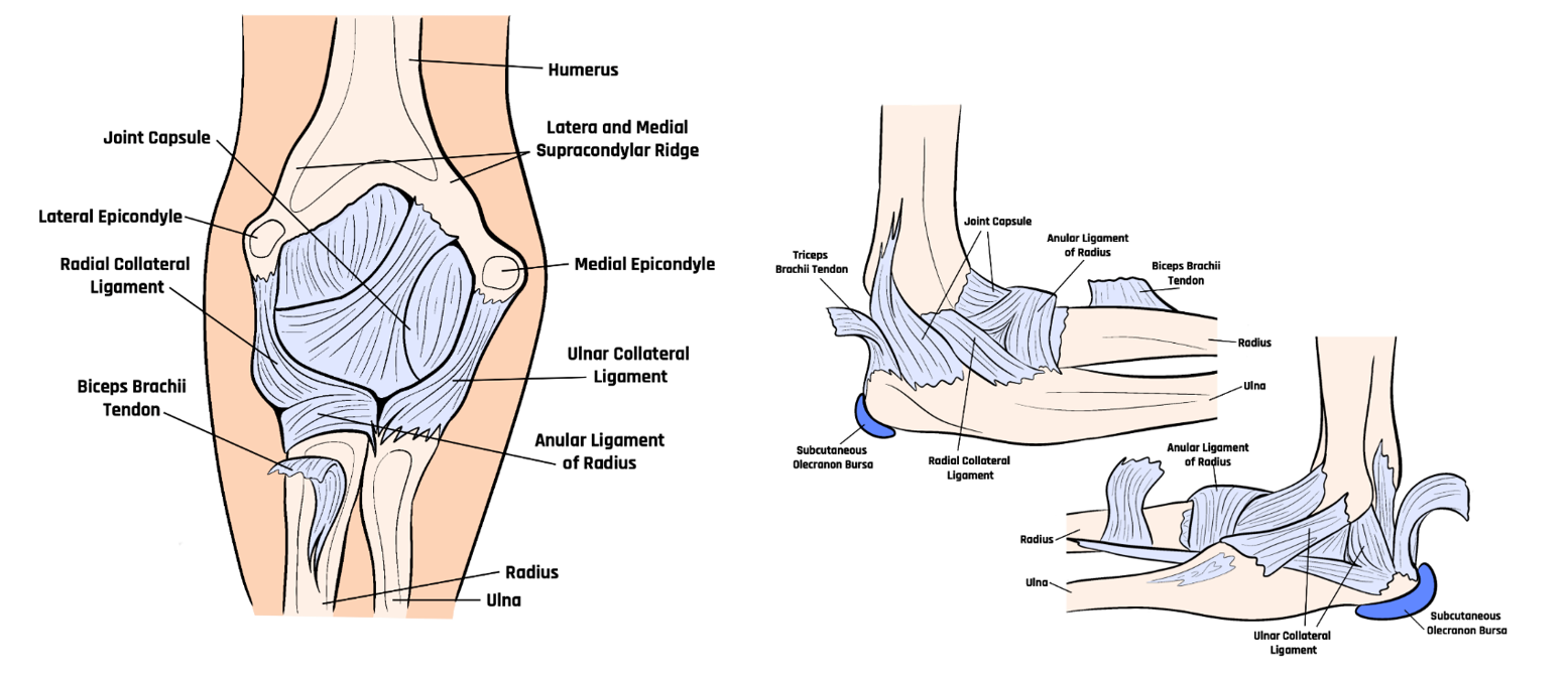
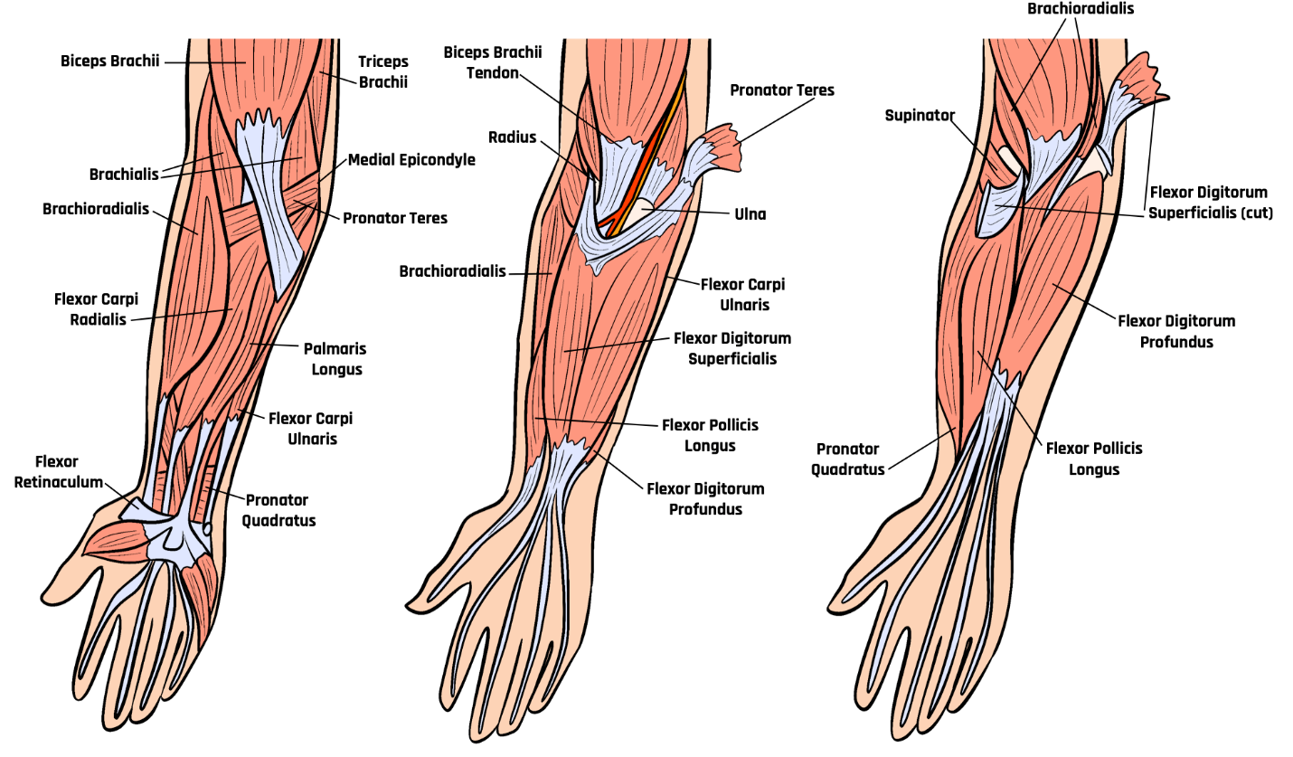
The entire elbow examination is usually accomplished with a linear transducer. Like all the other joints, the elbow is best evaluated in a quadrant approach: anterior, medial, lateral, and posterior. Figures 6-9 and 6-10 show the anatomical structures of the elbow.

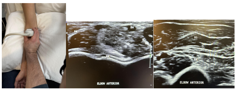
Anteriorly, look at the joint space for narrowing, cortical and cartilage irregularities, synovial hypertrophy, and effusion. Also evaluate the brachialis, biceps, median and radial nerves, and the brachial artery, as shown in Figure 6-11.

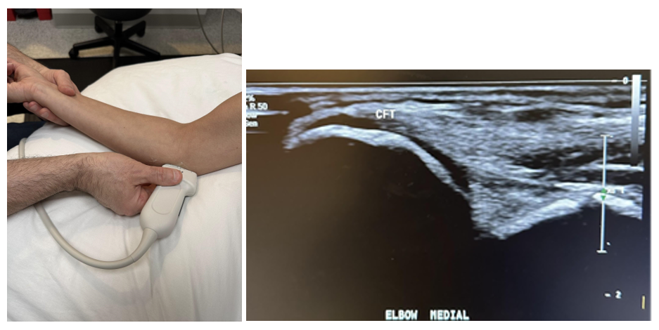
Next, the medial elbow evaluation is performed with the elbow in partial extension and the probe in a longitudinal axis, as shown in Figure 6-12. Evaluate the anterior band of the ulnar collateral ligament (UCL). It will have a characteristic triangular homogenous appearance as it spans from its attachment proximally to the humeral trochlea and distally to the olecranon. The common flexor tendon is superficial to the UCL and evaluated carefully at the insertion point of the medial epicondyle, since this is the site of medial epicondylitis. The pronator teres should also be examined for any evidence of tears, effusion, or synovial hypertrophy.^[10],^[11]

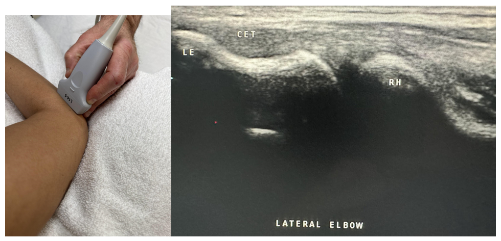
The lateral elbow is next approached with the elbow flexed at 90 degrees and the ipsilateral hand resting in pronation, as shown in Figure 6-13. A longitudinal probe placement is performed to evaluate the bony margins of the capitulum of the humerus and the radial head. Evaluate the radial collateral ligament complex and the common extensor tendon (CET). Closely evaluate the attachment of the CET to the lateral epicondyle, the site of lateral epicondylitis.

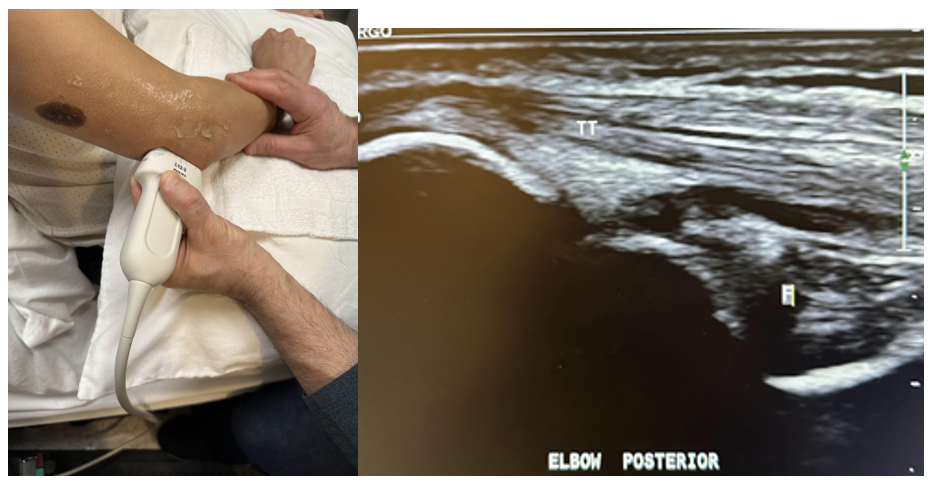
Finally, the posterior evaluation is performed with the elbow at approximately 90 degrees of flexion, as shown in Figure 6-14. Evaluate the triceps muscle and tendon, olecranon bursa, and the ulnar nerve within the groove between the medial epicondyle and the olecranon of the ulna. This can be a site for entrapment of the ulnar nerve, which should have an area of 7 mm or less.^[12],^[13]

6.7 Wrist and Hand Sonography

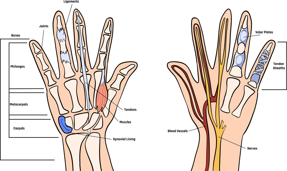
The wrist and hand anatomy involve superficial structures; therefore, the best approach is to use a high-frequency hockey stick transducer for better resolution. Figure 6-15 shows the anatomical structure of the wrist and hand.

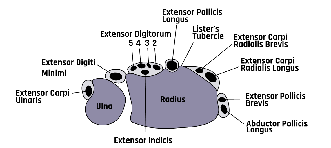
Start with the palm of the hand facing down. Identify Lister’s tubercle (see Figure 6-17) on the dorsum of the distal radius by digital palpation, and place the transducer on top of it in a transverse plane, as shown in Figure 6-16. This bony prominence separates the second and third extensor tendon compartments of the six in the wrist and helps with identification and orientation. Just radial to Lister’s tubercle is the second compartment containing the extensor carpi radialis brevis and the extensor carpi radialis longus.

With further radial movement, the first compartment on the side of the wrist is identified, which contains extensor pollicis brevis and abductor pollicis longus tendons. The first compartment is the site of de Quervain’s tenosynovitis. Evaluate each compartment from proximal to distal in both planes with active and passive dynamic maneuvers depending on the clinical concerns. Superficial to the compartments is the extensor retinaculum.

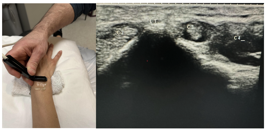
The third compartment is on the ulnar aspect of Lister’s tubercle and contains the extensor pollicis longus, as shown in Figure 6-17. Moving further toward the ulna, next to the third compartment, is the fourth compartment, which contains multiple extensor digitorum tendons and extensor indicis. Compartment five contains the extensor digiti minimi, and the sixth compartment contains the extensor carpi ulnaris, as shown in Figure 6-17. Evaluate each for any pathology.

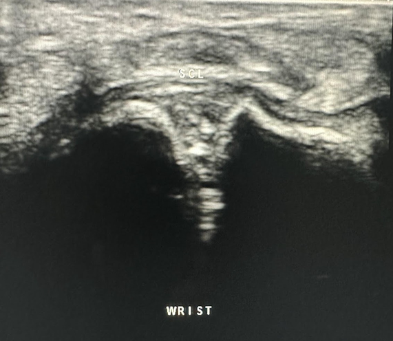
After evaluating each compartment, return to Lister’s tubercle in the transverse plane, and move the probe distally to the radiocarpal joint. The bone just distal to the radius is the scaphoid, and the lunate bone is next to the scaphoid in the ulnar direction. Between the dorsal aspects of both bones is a triangular area that represents the scapholunate ligament, which has a compact hyperechoic fibrillar echotexture, as shown in Figure 6-18. This is a common site for injuries from falls involving extended wrists that could result in a tear of the scapholunate ligament. It is also a common site for ganglion cysts.

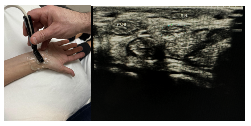
Now rotate the hand to evaluate the volar aspect, as shown in Figure 6-19. Evaluate the median nerve, flexor tendons, volar joint recesses, flexor carpi radialis, palmaris longus, and radial artery and the flexor tendons, pulleys, volar plates, collateral ligaments, and joint recesses of the fingers as clinically indicated. The median nerve is found between the flexor carpi radialis and palmaris longus. Place the transducer between these two tendons in the distal wrist crease in the transverse plane, and move the probe proximally as the honeycomb appearance of the median nerve courses radial to the flexor tendons and then moves ulnar and deep between the flexor digitorum superficialis and profundus. If the median nerve has a cross-sectional area of 12 mm² or greater, this suggests carpal tunnel syndrome. Also, a 2 mm² or greater difference in the cross-sectional area of the median nerve measured proximally at the level of the pronator quadratus and distally at the level of carpal tunnel has a 99% accuracy for carpal tunnel syndrome.^[14]

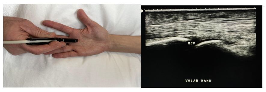
Finally, individual digits should be evaluated in the transverse and longitudinal planes using dynamic maneuvers as clinically indicated for the evaluation of pathology. There are five flexor tendon pulleys in the fingers, which are named A1–A5 and consist of annular ligament pulleys and cruciate pulleys—that is, the flexor tendon pulley system. The thumb only has two pulleys, which are labeled A1 and A2. When evaluating the pulley system in the digits, the A2 and A4 pulleys are most important in the sagittal plane, as shown in Figure 6-20. If pathology is present, this may demonstrate bowstringing and hypoechoic edema.^[15]

6.8 Hip Sonography

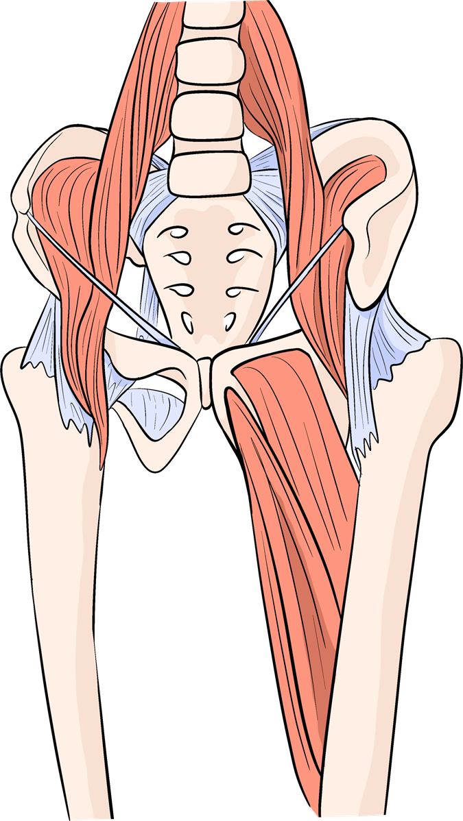
Figure 6-21 shows a schematic of the skeletal structure and tendons of the hip. The low-frequency curvilinear transducer is most appropriate for hip evaluation. Start with the anterior evaluation by having the patient supine with the ipsilateral leg in full extension and with slight external rotation, as shown in Figure 6-22.

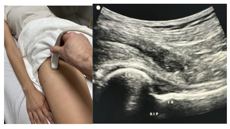
Superficial to the capsule is the potential space between the capsule and the iliopsoas muscle, which is the iliopsoas bursa. This is the largest bursa in the human body, and an iliopsoas bursitis would be considered an extracapsular effusion. Like hip capsulitis, iliopsoas bursitis can be approached with an injection—but more superficial. The iliopsoas tendon is then evaluated by placing the transducer in the longitudinal plane in line with the femoral shaft and medial. The iliopsoas is a conjoined muscle composed of the iliacus and the psoas major muscles, which attach to the intertrochanteric line of the femur. This is evaluated from proximal to distal in the longitudinal and transverse planes. Also, consider evaluating the femoral vessels and nerve, sartorius muscle, tensor fascia lata tendons and muscles, lateral femoral cutaneous nerve, and rectus femoris tendon and muscles. Dynamic hip maneuvers may also help evaluate for tears, subluxation, or dislocation.^[16]

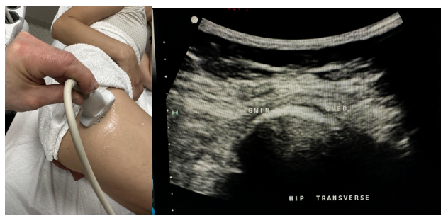
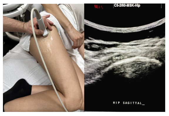
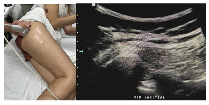
Now have the patient in the lateral decubitus position with the hip to be evaluated up in a flexed 20–30 degree position to examine the gluteus muscles and tendons, as shown in Figures 6-23 through 6-25. The gluteus minimus, which is deep to the gluteus medius, originates from the ilium between the inferior and anterior gluteal lines. It inserts onto both the anterior aspect of the capsule and via its long head onto the anterior surface of the greater trochanter. The gluteus minimus and gluteus medius work together to abduct and internally rotate the hip. Finally, the gluteus maximus starts in the posterior iliac crest and sacrum/coccyx, crosses over the posterior facet, and inserts into the proximal femur, as Figure 6-25 shows. It extends and laterally rotates the hip.

To visualize the tendons in the sagittal plane, rotate the probe 90 degrees and angle the beam anterior to posterior to visualize the gluteus minimus and posterior to anterior to visualize the gluteus medius, as shown in Figure 6-24, and the gluteus maximus, as shown in Figure 6-25.

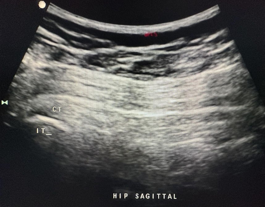
To evaluate the hamstrings, first identify the ischial tuberosity to locate the origins of the semimembranosus, biceps femoris, and semitendinosus tendons. Locate the conjoined tendons of the biceps femoris and semitendinosus, as shown in Figure 6-26. The semimembranosus lies deep and usually slightly inferior to the conjoined tendons.

6.9 Knee Sonography

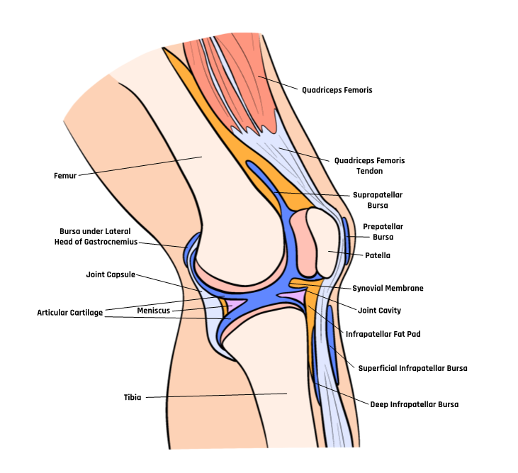
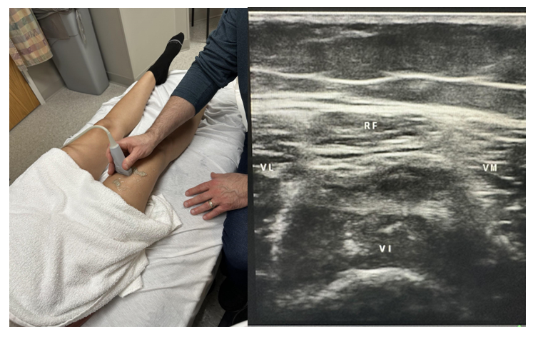
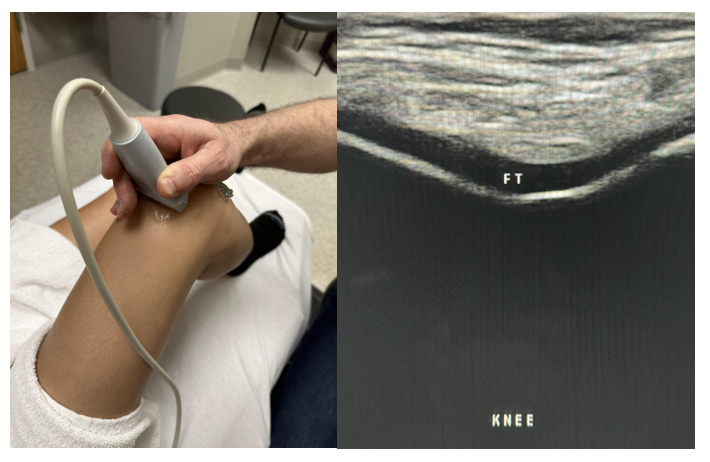
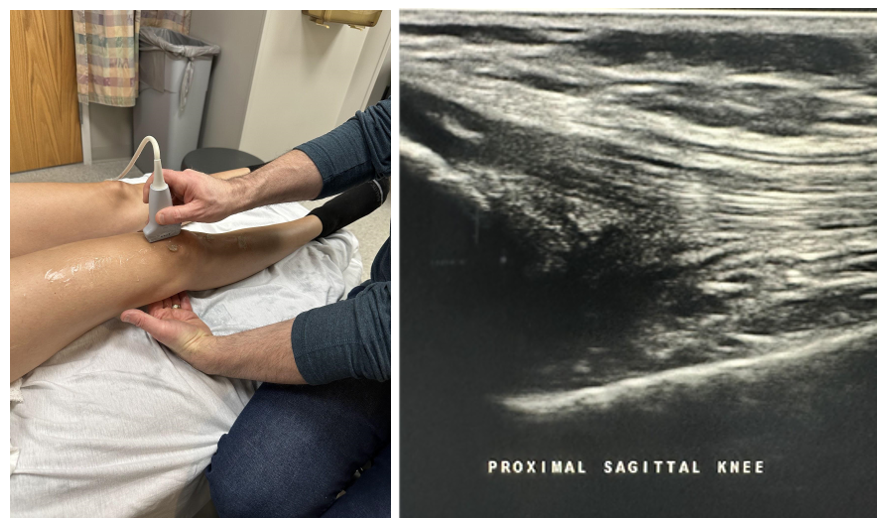
Start the evaluation by using a high-frequency linear transducer and having the patient in the supine position. The anterior evaluation starts in the suprapatellar area with the probe in line with the femur, as shown in Figure 6-28.

Evaluate the following structures from deep to superficial, starting with the bony cortex of the femur, the quadriceps muscles and fascial planes, the femoral trochlea, the prefemoral fat pad, the suprapatellar bursa, and the suprapatellar fat pad. Evaluate proximally from the quadriceps muscle to the distal area over the patella in the longitudinal and transverse planes, looking for any pathology such as effusion or tears, as shown in Figures 6-29 and 6-30. It is sometimes helpful to perform toggling and heel-to-toe maneuvers to fine-tune the anatomy and avoid anisotropy.

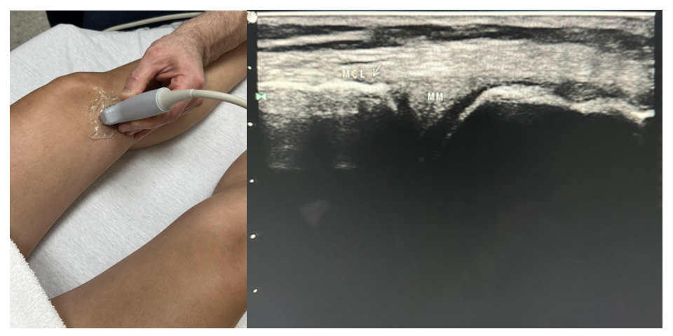
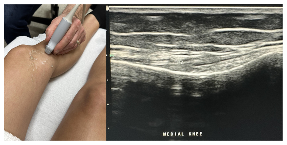
Next, slide the transducer medially, and evaluate the medial aspect of the knee joint from the femoral to the tibial condyles in the sagittal and transverse planes, as shown in Figures 6-31 and 6-32. Also, evaluate the medial collateral ligament and the medial meniscus in the joint space. As you move the transducer distally, evaluate the pes anserine complex for any evidence of injury or inflammation, such as pes anserine bursitis.

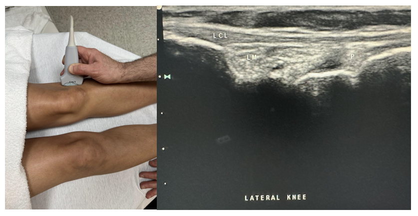
Next, slide the probe to the lateral aspect of the knee joint, and evaluate the joint space of the distal femur and fibular head, as shown in Figure 6-33. In the longitudinal and transverse planes, evaluate the peripheral margin of the lateral meniscus and the lateral collateral ligament from proximal to distal.

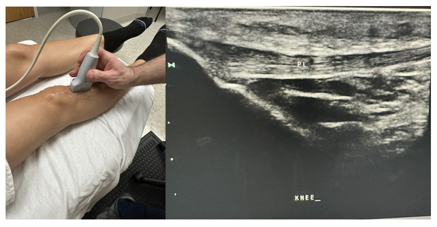
Next, scan the infrapatellar area in the longitudinal plane with the bony landmarks proximally of the femur and tibia joint space and distally of the proximal tibia, as shown in Figure 6-34. Keep light pressure on the probe to avoid compressing any possible fluid within the bursa. There are two bursae superficial to the patellar tendon near the patella and one deep to the patellar ligament in the area of the proximal tibia. Evaluate the patellar ligament, sometimes called the patellar tendon, which is the portion of the quadriceps femoris tendon that continues from the patella to the tibial tuberosity.

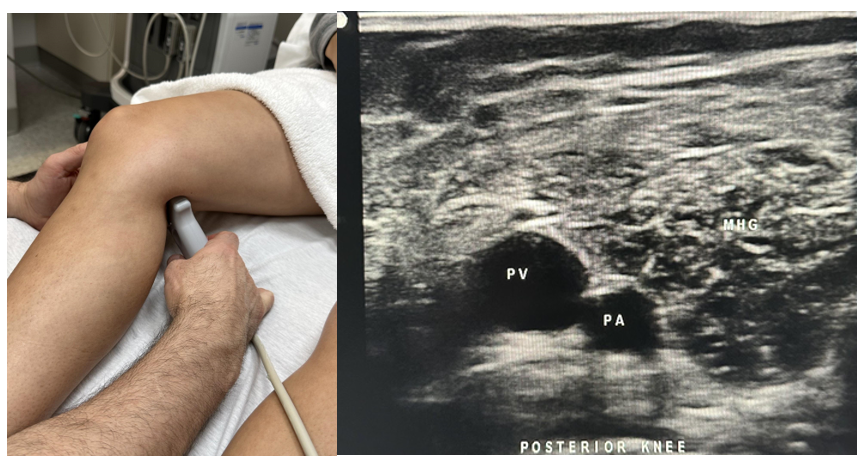
Finally, the posterior view of the knee is evaluated with the knee slightly flexed at 10–20 degrees, as shown in Figure 6-35. Many structures can be seen in the popliteal fossa, including the popliteal artery and vein. One important area to evaluate is the area between the medial head of the gastrocnemius muscle and the semimembranosus tendon, which is the usual site of a Baker’s cyst. This completes the knee evaluation.

6.10 Ankle and Foot Sonography

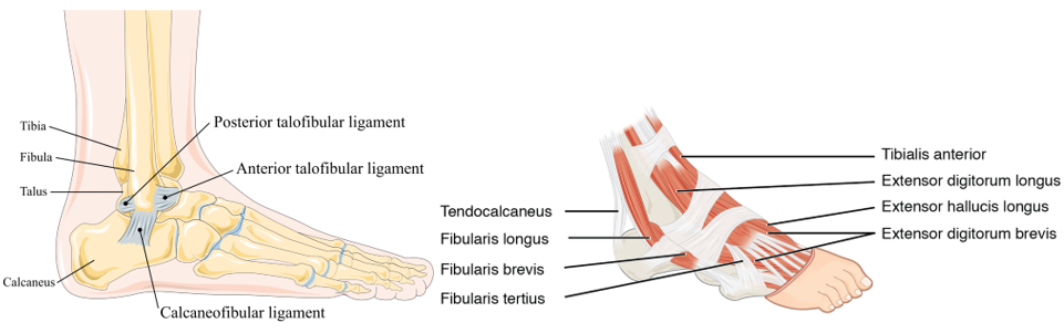
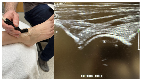
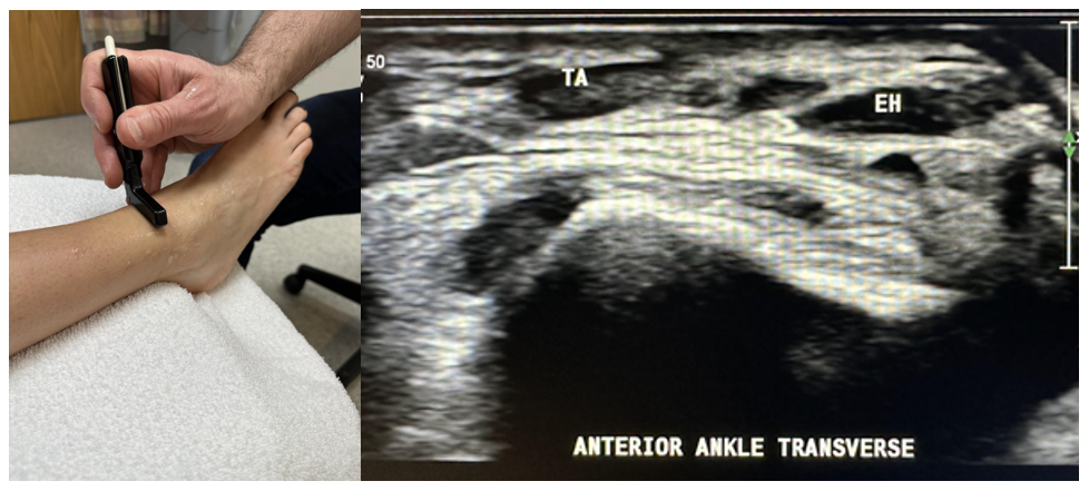
Figure 6-36 shows the anatomical view of the foot and ankle. The ankle and foot can be challenging to evaluate, since many structures require anatomic familiarity and detailed imaging. However, in general, a systematic approach is helpful. As with the other joint evaluations, a quadrant approach works best. Start with the anterior/dorsal evaluation by flattening the foot with an anterior longitudinal plane of the probe across the joint space of the tibia and talus, as shown in Figure 6-37. This provides an excellent focal point to sweep across the ankle joint to evaluate the muscles from medial to lateral: tibialis anterior, extensor hallucis longus, and extensor digitorum longus, as shown in Figure 6-38.

The subtalar joint is often of interest for evaluation and injection purposes. It is found in the longitudinal plane just medial to the lateral malleolus in the talus and calcaneus joint space.

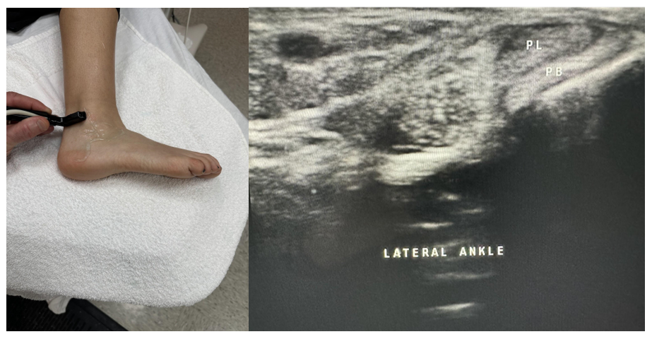
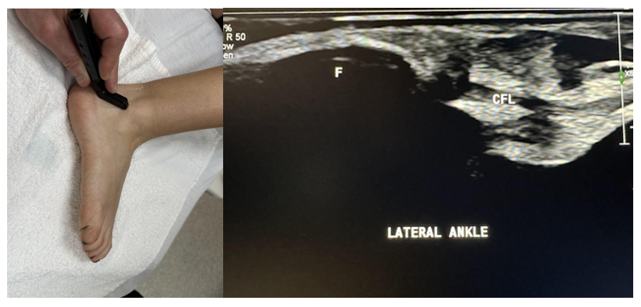
Evaluate from the proximal muscle to the tendon insertion points in the transverse and longitudinal planes as clinically indicated.^[17] Dynamic imaging is helpful to evaluate the integrity of the ligament. Now place the probe behind the lateral malleolus in the longitudinal plane with a posterior to anterior angle of insonation to evaluate the peroneus longus, which is superficial to the peroneus brevis. Evaluate both the longitudinal and transverse planes proximally and distally to their insertion points, as shown in Figures 6-39 and 6-40.

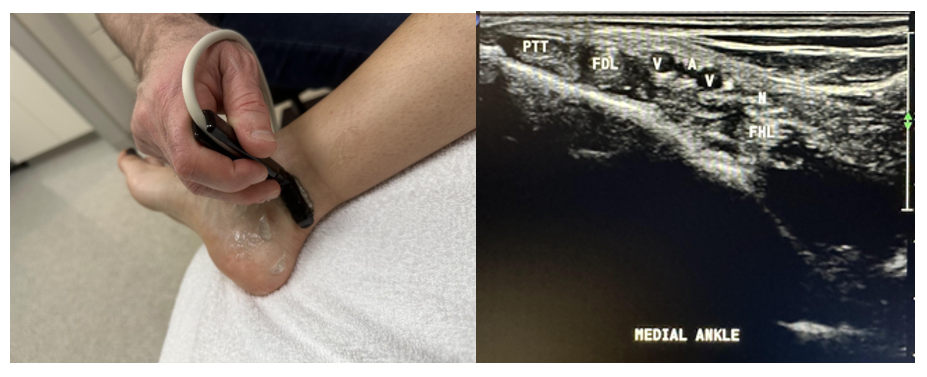
Place the probe in the transverse plane behind the medial malleolus to evaluate the medial side of the ankle and foot, as shown in Figure 6-41. Now we can evaluate the cross-sectional area of the structures in the tarsal tunnel. From medial to lateral, we have the Tibialis posterior tendon, flexor Digitorum longus tendon, posterior tibial Artery/Vein/Nerve, and flexor Hallucis longus tendon. Tom, Dick, And Very Nervous Harry is a commonly used mnemonic to recall these anatomical structures. This is important to evaluate for tarsal tunnel syndrome if clinically indicated.^[18]

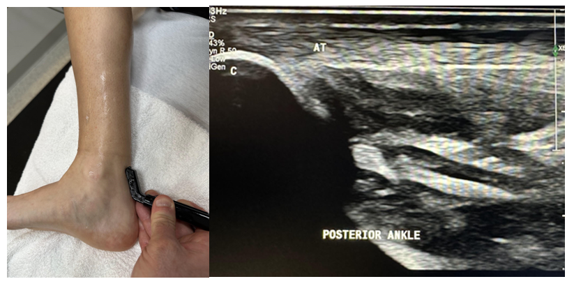
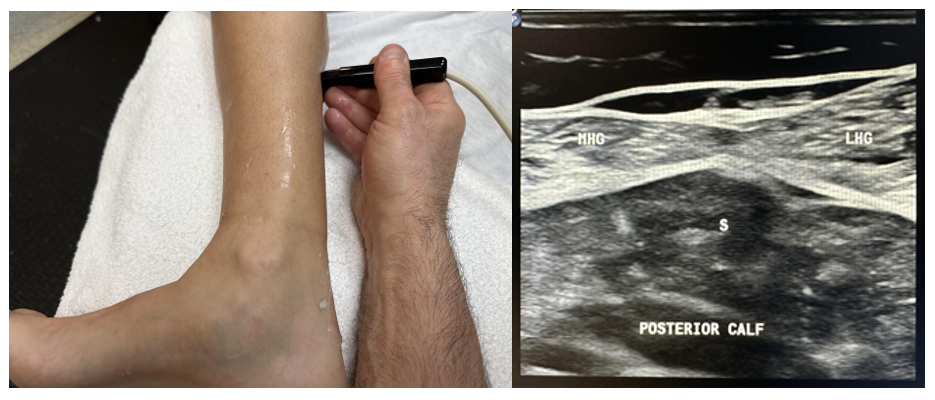
To complete the evaluation, look at the Achilles tendon in the transverse and sagittal planes from the proximal gastrocnemius and soleus muscles to the insertion into the calcaneus, as shown in Figures 6-42 and 6-43.

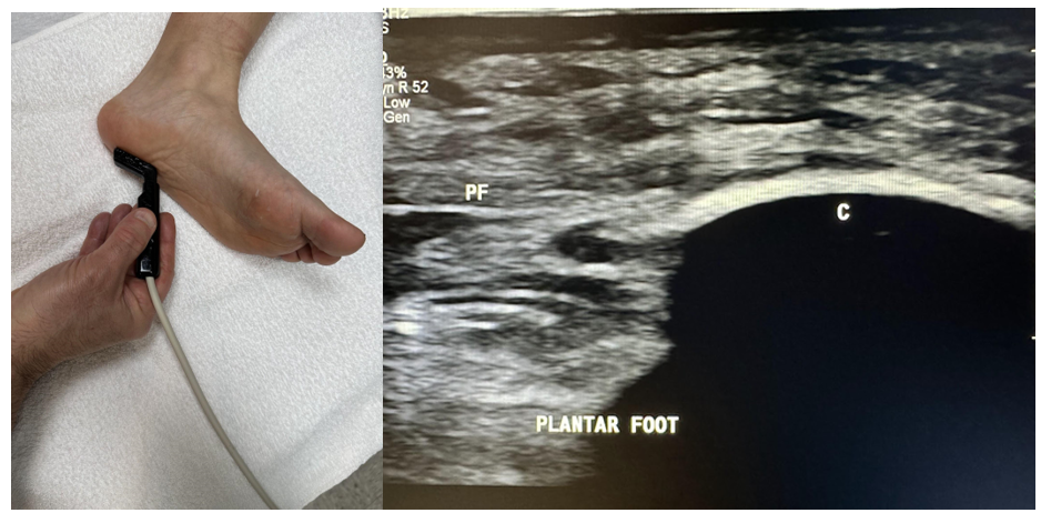
Finally, evaluate the foot’s plantar fascia in the longitudinal plane, as shown in Figure 6-44. The thickness at the insertion to the calcaneus should not be more than 4 mm, which would be suggestive of plantar fasciitis.