
5 Form and Function
Kelly M. Diamond and Vanessa K Hilliard
Focus Questions—to Guide Your Reading of This Chapter
- What are the most basic metrics of anatomical forms?
- How do we quantify function?
- Why do some anatomical structures grow to different proportions compared to others in the same organism? In different organisms?
- What are Newton’s three laws of motion? How are they relevant to our consideration of functional anatomy?
- Does form always relate to function?
5.1 Introduction
Oftentimes, learning anatomy is approached with a memorization mindset: There are lists of structures, and one just needs to memorize their names and where they are. However, we find that such an approach robs the study of anatomy of its richness, because it reduces complex, integrated bodies into stagnant, stand-alone “parts,” with little acknowledgment of their roles within the body. By extension, this lack of functional recognition also leaves us with little explanation of the “why” behind anatomical diversity across vertebrate taxa, which (in our opinion) is one of the most fascinating questions in all of biology.
In this chapter, we’re going to consider the relationship between form and function and some of the factors that influence this dynamic. We’ll first define what we as anatomists mean by form and how we measure it. Then we will move on to the important question: What is function? And in addressing this broad question, we’ll take a peek into the fields of functional morphology and comparative biomechanics, which aim to explain how bodies work and are deeply rooted in the study of anatomy. Generally speaking, these fields of study seek to understand things like why we switch from walking to running at certain speeds, how flying critters actually fly, and how the structure of different anatomical parts makes things like feeding and locomotion possible in different types of environments. In other words, we start with normal activities of ordinary organisms and ask “how?” and “why?” And in order to answer those questions, we need to draw on aspects of the physical world. In short, this is a field of biology that uses principles of physics and engineering in order to understand how bodies work. There are both advantages and disadvantages when approaching biomechanics and functional morphology. One distinct advantage is our familiarity with the phenomena that we’re trying to explain—we experience things like gravity every day—though we may not always be consciously aware of it. And this everyday experience gives us an innate sense of reality when addressing functional questions. However, the downside is that explaining and quantifying the physical world requires us to use tools and draw on concepts that are not often well used (or even present, in some cases) in the standard biologist’s intellectual toolbox. So in this chapter, we’re going to introduce you to some of those tools and concepts so that you are well equipped to think about anatomy in a functional context, and we will answer the “how” and “why” questions that naturally arise in the study of comparative anatomy.
5.2 What Is Form and How Do We Measure It?
It might seem obvious that form is the anatomy that you are aiming to learn with this book. However, before we dive into our discussion of function, we first must discuss how we, as anatomists, define the term form and how we measure it. For each of these forms, you will learn more detail in later chapters. Our goal for this section is to introduce the basic building blocks and how they relate to each other.
Anatomical Forms
Vertebrates experience forces that their structural systems, or anatomical forms, must withstand. Some of these forces are produced internally by an organism, while other forces are produced outside of the organism, by environmental factors. There are many different types of form-function relationships. For this chapter, we will mainly focus on two categories of form-function relationships: those associated with locomotion and those associated with feeding.
For both categories, the underlying anatomical form, upon which forces act, is the vertebrate skeleton. Since skeletal elements are relatively stiff structures, movement of the skeleton occurs at joints, where different skeletal elements come together. Specialized connective tissues, called ligaments, connect the skeletal elements together across a joint. The points at which two skeletal elements interact with each other are called points of articulation. Normally you can observe these points on the skeleton because the cartilage or bone is smoother where they articulate, or rub together.
Another anatomical element that we need to consider as part of our anatomical form is the skeletal muscles, which contract when stimulated by motor neurons. Skeletal muscles are connected to skeletal elements via other specialized connective tissues, called tendons. As these muscles contract, they will produce forces that act on the tendons, which in turn act on the skeletal elements, causing movement at the joints.
Anatomical Materials
How does the material that a critter is made of impact the way it works? Anatomical materials, or biomaterials, differ from architectural materials due to the requirements for anatomical structures to change in size and shape over time while still maintaining their durability.
The beauty of, and the trouble with, bodies is that classifying the stuff an organism is made of can be somewhat difficult. One way to approach this idea is hierarchically, based on chemical composition. But the difficulty with this approach is that chemical composition doesn’t necessarily correspond with mechanical properties—and for our purposes, that’s not super useful. So instead of classifying things chemically, we’ll classify solid materials based on their mechanical behavior, which describes how well a material maintains its shape. This way of classifying materials puts biomaterials in one of three categories:
- Tensile materials, which are good at resisting stretching;
- Pliant materials, which are relatively easy to deform but return to their original shape when the load is removed; and
- Rigid materials, which strongly resist deformation and don’t return to their original shape after deformation.
But this is still a little abstract. What types of anatomical forms actually represent these three categories of materials? Let’s begin with tensile materials. Tensile materials function by resisting pulling forces or tensile stress. They are, in essence, biological ropes. But even though we can think of these as biological ropes, they aren’t always used as ropes and are often found as part of other materials. When we look at living organisms, we find four distinct kinds of tensile materials: silk, collagen, cellulose, and chitin. And since we’re concerned with vertebrates and human bodies in the context of this book, collagen is the major one on this list that you’ll want to pay attention to. Collagen is a protein, and it can be found in fairly pure form in our own tendons (Figure 5.1A). But collagen can be found in lots of other structures as well, often as one element of a composite material, materials made up of more than one thing. Some examples of composites that contain collagen include things like skin, bone, muscle, and the walls of blood vessels (most notably arteries).
Pliant materials will deform somewhat when stressed, meaning that they’ll stretch or squeeze some, and will return to their original form after the stress is removed. Examples of pliant materials include rubber-like proteins and pliant composites. Rubber-like proteins can be drastically distorted and then rapidly return to their original shape. The most familiar of these is probably elastin (Figure 5.1B), which can be found in your own skin and arterial walls. Rubber-like proteins are all functionally similar in that they are stretchier than tensile materials. Pliant composites are materials that only exist as, well, composites (hence the name), and this is a pretty varied group of stuff. Within the classification of pliant composites, you’ll find such diverse materials as the jelly of jellyfish and sea anemones, the cartilages of our ears, nose, and intervertebral disks, our skin and arterial walls, and even the mucus that provides traction for snails and slugs!
The third class of materials is rigid materials. These are materials that strongly resist any kind of deformation, and all rigid materials are composites. Examples of familiar rigid materials include things like bone (Figure 5.1C), keratin, and enamel.

Figure 5.1—Anatomical examples of the three different categories of biomaterials. Tensile materials (A) resist pulling forces, as seen in the collagen fibers in a muscle tendon. Pliant materials (B) such as the elastin in your skin are easy to deform but bounce back to their original shape when a force is removed. Rigid materials (C) strongly resist any kind of deformation, as seen in bone tissue.
Measuring Form
If we want to quantify the form an organism has, we first need to define some basic physical quantities. We will then use those basic physical quantities to derive additional physical quantities that tell us more about the form itself and how that form could be expected to function. Finally, we will discuss how we use different reference systems to quantify and compare these different metrics.
Basic Physical Quantities
The two most basic physical qualities that we as anatomists use to define form are length and mass. Length (l) refers to the distance between two anatomically defined points. Our second basic physical quantity is mass (m), which is the total amount of stuff that makes up an organism. A third basic physical quantity that is not directly related to form, but is used to quantify how forms move, is the quantity of time (t), which is used to quantify the duration of a particular event. These three quantities are used to derive additional physical quantities that describe form and associated metrics of function.
Derived Physical Quantities
Our first set of derived physical quantities, which are defined relative to the length of a form, will help us further quantify the form of an organism. We will use a square or cube, with length (l) equal to the length of one side of the cube, as our example form to show how length is used to define each quantity (Figure 5.2). Area (A = l2) is the amount of space a two-dimensional object takes up. Moving into three-dimensional space, volume (V = l3) is the amount of space that a three-dimensional object takes up. Surface area (SA = 6 l2) is the amount of space covering the outside of an object. The derived quantity that quantifies how much mass is in each unit of volume is density (D = m/V).
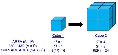
Figure 5.2—Area, volume, and surface area of two cubes. In this example, the length (l) of Cube 1 has been set to 1, which yields an area of 1, a volume of 1, and a surface area of 6. When we double the size of the cube (l = 2), we see how area increases 4-fold, volume increases 8-fold, and surface area increases 24-fold. So a simple change in length can have a radical effect on other derived physical quantities.
Our next set of physical quantities help us understand the forces associated with movement of an organism or parts of an organism. We can start to get a sense of these relationships by asking questions that help us describe motion. For example, some of the questions we can ask include (Note: This is not an exhaustive list):
- How hard is it to move the organism? This is described by force (F), calculated as mass (m) times acceleration (a) (F = ma). Force is related to weight (w), because weight is simply mass times acceleration due to gravity (often abbreviated as g). In Figure 5.3A, the weight of the sitting cat is the mass of the sitting cat times the acceleration due to gravity. If you wanted to pick up the cat, it would take a force opposing the weight of the cat.
- OK, we have a force, but how intensely is the force being applied? We can describe this as either stress (σ) if the force is internal, as it would be on a bone when a muscle pulls on it, or a pressure (p) if the force is applied from an external source outside of the structure, such as when the atmospheric pressure changes depending on your altitude. Regardless of how force is applied, stress and pressure both essentially describe the relationship between force and area (force divided by area, F/A, to be precise). Stresses and pressures both cause structures to deform to some degree (Figure 5.3B), and this measure of deformation as a result of stress or pressure is what we call a strain (e). Strain is calculated by taking the change in length of the structure and dividing it by the structure’s original length.
- How far does the force move the organism? This question asks about work (W), which is force times distance. The capacity to do work is energy!
- How fast is the organism moving? Once a strong enough force is applied to an organism, we can start to talk about motion. First we can measure speed, which is determined by taking the distance traveled (which is another length) and dividing it by time. In Figure 5.3C, this would be the amount of time it takes the tortoise and the hare to move from the starting line to the finish line, divided by the distance between the starting line and the finish line. We can even take this a step further and describe the direction the organism is moving if we have that information, which would give us the organism’s velocity (v)—that is, speed in a specific direction. Since the race in Figure 5.3C is only from the starting line to the finish line, we could describe the movement of the tortoise and the hare as their velocity.
- How fast is velocity changing? The answer to this question is acceleration (a = v/t), which is determined by dividing velocity by time. In Figure 5.3C, the tortoise accelerates at the start of the race and decelerates at the end of the race, but in between it maintains a constant speed, or has no acceleration, while the hare accelerates and decelerates with each jump it takes during the race.

Figure 5.3—How forces work. Forces must overcome the weight of an object in order to move an object (A). Forces can be applied from internal stressors (σ) or external pressures (p) to cause a deformation of the shape, measured as the strain (e) on the object (B). Forces can cause objects to move, or do work, such as when the tortoise and the hare use energy to race (C), both animals use different velocities (dotted lines) and accelerations as they move from the start to the finish line.
Reference Systems
Now that we’ve defined different physical quantities, we need to discuss how we compare those physical quantities. For each quantity, there is a unit that is used to standardize how each of these measures is compared. Table 5.1 provides some examples of such standardized units. Many of these units can be plotted to visualize differences between groups or changes over time. To make these plots, we often use a Cartesian coordinate system, where points are plotted in a horizontal (x) axis, vertical (y) axis, and for three-dimensional objects, a third (z) axis that is perpendicular to both the x and y axes.
Table 5.1—Standardized units for form-function quantities
|
Metric |
Abbreviation |
Unit |
|---|---|---|
|
length |
l |
meter |
|
mass |
m |
kilogram |
|
time |
t |
seconds |
|
force |
F |
Newtons |
|
pressure and stress |
P and σ, respectively |
Pascal |
Before moving on to function, you may have noticed that force keeps emerging as a recurring theme in many of the derived physical quantities listed above. This is because forces are absolutely critical to understanding the motion of organisms. Forces are analyzed as vectors, meaning that they have both magnitude and direction. To visualize this, think about how we describe a force: If I try to pick up the cat in Figure 5.3A, I’m exerting a force that must be larger than the weight of the cat in the opposite direction of the weight of the cat. The amount of force I use to pick up the cat is the magnitude or size of the force I’m exerting, and up is the direction in which the force is being applied. But what does this mean if we’re trying to understand how organisms or their parts move? How do we figure out how a force will affect a structure? These are the concepts we will cover in our next section on function.
5.3 What Is Function and How Do We Measure It?
So what is “function”? In general, function can be defined as how things work, and in the context of comparative anatomy, we can frame this definition specifically as how organisms work. And oftentimes function revolves around motion: either making things move or resisting movement. There are four primary, overarching factors that affect organismal function:
- Size and shape
- Mechanics
- Environment
- Phylogeny/evolution
The last of these—phylogeny—is largely covered elsewhere in this book (e.g., in the nonvertebrate chordate in Chapter 2 and to a certain degree in each of the anatomical systems chapters), so we won’t spend much time on that particular factor here. For the remaining three factors, we will explain basic concepts here, and then in our final section of this chapter, we will discuss how these concepts are used to study form-function relationships in the real world.
Consequences of Size and Shape
For every type of animal there is a most convenient size, and a large change in size inevitably carries with it a change of form.
—Haldane, 1927
The quote above eloquently describes how as the size of an organism changes, the demands on different body parts change disproportionately. In anatomy, we describe this as differences in scaling. All vertebrates are three-dimensional beings, meaning that they have length, width, and height.
All vertebrates also change body size, either through individual growth or as changes among species through the course of evolution.
Isometric Growth
Let’s consider growth first, which involves dimensional change. As the individual grows, each of the dimensions (i.e., length, width, height) can change in equal proportion. This type of increase would produce animals that are geometrically similar and represent what we refer to as isometric growth (“iso” = same, “metre” = measure or, in this case, dimension).
This can be a little bit abstract to wrap one’s mind around, so to help illustrate this concept in a simplified manner, we’re going to examine a cube-shaped organism and see how things change as it undergoes isometric growth (Figure 5.4). So let’s begin with our cube-shaped organism, and we’ll define its anatomy as 1 cm in length, width, and height. Now if our animal grows twice as large, it will double each of these dimensions, so length, width, and height each become 2 cm. So far, so good. But what does this change in length do to the organism’s surface area and volume? Well, length is twice as large after growth, but area is four times larger and volume is eight times larger! What this demonstrates is that a doubling in length doesn’t just double the area and volume—it actually produces a fourfold increase in area and an eightfold increase in volume (which can be equated to an eightfold increase in mass). These are very big changes. But aside from a cat sitting in a cube-shaped box, are there really any cube-critters out there? How does this translate to living organisms? Well, this pattern holds true for other shapes as well, not just cubes; as you can see in Figure 5.4, dimensions change for spheres and cylinders (which are much more realistic approximations of vertebrate body shapes—most mammal bodies tend to be spherical, whereas fish, amphibian, and reptile body shapes tend to be cylindrical).

Figure 5.4—Scaling relationships between size (l = length, r = radius, h = height), surface area (SA), and volume (V), in 3D cubes, spheres, and cylinders.
Even in these simple forms, the surface–area–to–volume ratio as depicted in Figure 5.4 has some pretty major consequences for function. For example, in endothermic (self-heating) vertebrates, heat loss scales with surface area, but heat generation scales with volume. What this means is that smaller animals need a relatively higher metabolism and to eat relatively more food, to maintain their body temperature compared to larger animals, because their surface-area-to-volume ratio means they lose more heat to their environment. We can also see how the surface-area-to-volume ratio interacts with environmental variables by looking at body shapes of animals that live in cold versus warm climates. In cold habitats, endotherms want to maximize heat production (volume) and minimize heat loss (surface area), so they tend to be more sphere-shaped with shorter extremities to maximize their surface-area-to-volume ratio—for example, the snowshoe hare (Lepus americanus) seen in Figure 5.5. Whereas in warmer climates, endothermic animals tend to be less sphere-shaped with longer extremities to maximize heat loss. Note the relatively longer limbs and ears in the jackrabbit (Lepus californicus) compared to the snowshoe hare in Figure 5.5.

Figure 5.5—Surface-area-to-volume ratios in the wild. Snowshoe hares (left) live in colder climates and are more spherical to maximize their volume and minimize their surface area, while jackrabbits (right) live in warmer climates and have proportionally longer limbs to maximize their surface area, allowing for greater heat loss.
Allometric Growth
The surface-area-to-volume ratio is one driver that can cause different parts of an animal to grow at proportionally different rates through development or over evolutionary time. Now we’re going to focus on an example that shows how changes in proportion affect the way in which the skeleton supports body mass. Consider a bone in the leg. If this bone is loaded and the stress of that load becomes too high, the bone will break. If an animal increases in size isometrically, how will the stress that results from an increase in size change as animals get bigger? We know that force is proportional to mass (F = ma) and that the acceleration in this equation is acceleration due to gravity. So limb bone stress should increase as animals get bigger, because stress = force divided by area (stress = F/A).
In fact, there was a time when researchers used this relationship to predict a maximum size for animals using limbs. However, organisms have found a way around the maximum size limitations imposed by isometric growth. Indeed, animals can also change shape as they grow or through the course of evolution—and this change in shape alongside a change in size is called allometry. In other words, if isometry is growth with geometric similarity, then allometry is growth without geometric similarity.
For example, if we were to consider our leg bone example again, what if the diameter of the leg bone increased twice as quickly as the length? If this happened, the bone would become relatively thicker with increasing size, thereby increasing the cross-sectional area of the bone. Because we know that stress = F/A, an increase in cross-section area actually helps limit increases in stress as the animals get bigger. And we can evaluate whether animals show allometry by simply measuring their dimensions, plotting the relationship, and calculating the slope of the plot. For isometric length-mass relationships, we’d expect the slope of the line to be 1/3. If the slope of the line is greater than 1/3, that tells us that the diameter of the bone is increasing faster than body mass and therefore is helping to accommodate increases in stress. In contrast, if the slope is less than 1/3, that means that body mass is increasing at a faster rate than cross-sectional area, and in this situation, an animal can be in pretty big trouble (because mass will quickly exceed the limits of the bone and lead to structural failure). These relationships help to explain why people don’t grow indefinitely and why we don’t see humans 50 feet tall walking around and terrorizing major cities (as depicted in some 1950s horror flicks and even the 1990s movie Honey, I Blew Up the Kid; see Box 5.1).
Box 5.1—Allometry of Movie Monsters
Why can’t 50-foot-tall movie monsters exist? Thankfully, the reason we don’t have to avoid the Godzillas and King Kongs of the movies is because for each unit increase in length or height, an animal’s or human’s body volume increases eightfold (Figure 5.4). But recall that bone cross-sectional area increases like an area, so for each increase in length, it only increases fourfold (assuming no change in shape). What this means is that if we take a 5-ft-tall person and turn them into a 50-ft-tall person with no other change in body proportions, that individual will be 10 times taller, their bone cross-sectional area will be 100 times larger, and their mass will be 1,000 times larger. And on the surface, these values may appear OK, but what this really means is that this kind of growth would put 10 times more stress on the person’s bones than the bones are actually capable of withstanding! In essence, as animals get bigger, forces on bones increase faster than the body’s ability to resist forces, unless proportions of the bones change (i.e., unless there’s allometric growth).
Question to think on: Using the graph provided in Figure 5.6, what do you think could be the maximum size of our hypothetical “movie monster”?
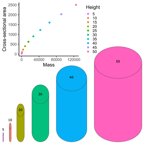
Figure 5.6—Allometry of movie monster bones. The graph shows the relationship between body mass and bone cross-sectional area. The points in the graph are color coded for movie monster height. The cylinders below the graph show a visual relationship between height and diameter for several of the color-coded points on the graph. The numbers above each cylinder represent the represented height.
Consequences of Mechanics
The field of biomechanics applies the physical principles of mechanics to the living world. We will start off this section by reviewing Newton’s laws of motion. Then we will use those laws to describe the simplest type of machine, the lever system. We will then discuss how lever systems are loaded with different forces to cause movements, a field of biomechanics called kinematics.
Newton’s Laws of Motion
- The law of unbalanced forces. This law tells us that a body at rest stays at rest or a body in uniform motion in a straight line stays in uniform motion in a straight line unless a force is applied to it. In other words, things that are still stay still, and things that are moving stay moving unless an outside force acts upon them.
- In Figure 5.7, if neither the triceps muscle nor biceps muscle is shortening, then the arm will remain at rest. If either muscle is shortening, then the forearm will move in the direction that the muscle pulls it until the muscle stops shortening.
- The law of acceleration (F = ma). This one should look familiar—it’s the same definition we provided for force earlier in this chapter! What this law tells us is that acceleration is proportional and in the same direction as the applied force.
- In Figure 5.7, the force that either the triceps or biceps muscle can produce is equal to the mass of the muscle and the rate at which that muscle can shorten to cause the extension or flexion of the forearm.
- The law of action and reaction. This law tells us that when one body exerts a force on another, the second always exerts a force back on the first in the form of a reaction force. What’s more—these two forces are equal in magnitude, opposite in direction, and act along the same line.
- This law explains how the musculoskeletal system works to allow our bodies to move. When the biceps muscle contracts (Figure 5.7), the muscle is exerting a force on the radius bone in the forearm. The radius and the rest of the connected forearm react to that force by flexing the forearm at a rate proportional to the force produced by the biceps.
- It’s worth mentioning here that this third law tells us that forces are still exerted on an object even if the object doesn’t move! If in Figure 5.7 the person was trying to pick something up that was extremely heavy—say, a 1,000-lb dumbbell—the person’s bicep would still be exerting a force (Fb) on the dumbbell, and the dumbbell would still be exerting a force on the muscle, even though neither would be moving! In this situation, the forces are in balance, and the system is said to be in equilibrium.

Figure 5.7—Newton’s laws of motion applied to muscle movements. The force of the triceps muscle (Ft) controls the extension of the forearm, and the force of the biceps muscle (Fb) controls the flexion of the forearm.
Lever Systems
In order to apply these laws of motion, we need to next think about how anatomical forms work together to create motion. In moving parts of the body, what we often observe are bones and muscles working together as lever systems. Now thinking of parts of the body in terms of simple machines may seem a little strange at first, but in fact, relating biological systems to familiar, simple machines can actually be quite helpful in understanding how they work. So before getting into specific lever examples of the vertebrate musculoskeletal system, we first need to introduce a basic lever, its parts, and how it works.
We’ll begin by considering a teeter-totter (or seesaw, if you will). This familiar playground toy is the perfect reference, because it is simply a big lever (Figure 5.8A). The two benches are the lever arms, or the components of the lever where force enters the system and exits the system (in the form of motion); the hinge, or the point about which the lever arms pivot, is called the fulcrum. On one side of the fulcrum, force will be loaded via the in-lever arm (Lin), and on the other side of the fulcrum, force will be output via the out-lever arm (Lout). The force that the movement of the Lout in general works to move an opposing force called a load, but more on that in the next section.

Figure 5.8—Lever systems. A basic lever system (A) shows the fulcrum (orange), separating the two lever arms, with the in-lever on the same side as the input force (Fin in pink), the out-lever on the same side as the output force (Fout in blue), and the loading force represented by a cat here in purple. Colors are consistent throughout the figure. A comparison of the lever system of a runner versus digger forelimb (B). The three classes of lever systems with biological and basic diagram examples (C).
Let’s bring back Newton’s third law here—for every action, there is an equal and opposite reaction. What this means is that the forces (F) transmitted through lever arms (L) can be expressed as
Fin × Lin = Fout × Lout
This also means the relative lengths of the lever arms of the lever system can impact whether a lever is built for strength or built for speed. When the Lin is relatively long compared to the Lout, like it is in a crowbar, a lever can move a large load with relatively little force input; these levers have a mechanical advantage (Figure 5.8B). When the Lin is relatively short compared to the Lout, a lever will require more force, but it can move a load a given distance quickly; these levers have a velocity advantage (Figure 5.8B). So velocity (V) and lever arm length (L) have an inverse relationship, which can be expressed as
Lin × Vout = Lout × Vin.
But why are levers important in the body? Let’s consider our lower leg and the calf muscle as an example (Figure 5.8C). The muscle that pulls on the back of the foot when it contracts (i.e., gastrocnemius) is inputting force (Fin), causing the foot to extend. Notice here that the foot actually has a small posterior extension—this is the heel bone (i.e., calcaneus) where the tendon for the calf muscle attaches. What this means is that the force from the muscle is actually acting at a distance from the ankle joint rather than on the ankle joint directly. Any force acting a given distance from a joint will tend to cause rotation about that joint, so the joint becomes a point of rotation. The distance between where the force is acting and the joint that is rotating is called the moment arm (r), which is the same thing as a lever arm. The process of a force acting at a distance from a point is called a moment and can be calculated by M = r × F. So when the calf muscle contracts, it will pull on the heel and cause rotation about the ankle—this is what’s happening in your lower leg when you point your toes (or really any time you extend your ankle)!
Animals that move in different ways through their habits tend to have skeletons with different lengths of lever arms. For instance, if we compare the elbow joints of animals that dig versus animals that run, we can see how the lever system of the elbow links form and function (Figure 5.8B). Looking first at diggers, they tend to have relatively long in-levers at the elbow (i.e., the in-lever is long compared to the length of the out-lever) in order to confer mechanical advantage, whereas runners have relatively long out-levers in order to confer velocity advantage (i.e., the in-lever is short compared to the length of the out-lever). This is because digging limbs need force, whereas running limbs need velocity.
There are a few different classes of levers, each distinguished by the relative position of the fulcrum and the load (Figure 5.8C). First-class levers are those in which the fulcrum is located between the point of applied force and the load to be moved; as such, the direction in which force is applied is opposite to the direction of motion produced. Your neck joint, when involved in lifting the chin, can be classified as a first-class lever, because the Splenius capitis muscle originates on the vertebrae and functions to pull the occipital region of the skull dorsally. In a second-class lever, the force application and direction of motion are on the same side of the fulcrum, which is located far from the applied force, with motion produced between the force and fulcrum. An example of a second-class lever would be your foot as you rise up on tiptoe. Third-class levers also have force application and produce motion on the same side of the fulcrum, but this lever is distinguishable from second-class levers in that the force is closer to the fulcrum that the movement produced. An example of a third-class lever in the body is the action of a biceps curl (i.e., elbow flexion).
Loads
At this point, we’ve mentioned the concept of “loading” a couple times, but we haven’t really explained what loading is yet. A loading regime (Figure 5.9) is the way in which a force or set of forces is applied to a structure. Bringing Newton back into the discussion, in general, when a load is applied to a structure, the structure will either resist movement (Law 1) or move (Laws 1–3). Loads can be applied to structures in several different ways. Tensile loads, or when a load is applied in tension, are loads that result in pulling along the long axis of a structure. This will result in the lengthening and narrowing of the structure’s material (to help you visualize, think about what happens when you stretch a rubber band). Compression is the opposite of tension; this is a loading regime in which forces applied in opposite directions produce a squashing load along the axis of a structure; this results in a shortening and widening of the material. Shear is a loading regime produced when there are two opposing parallel forces, but they are not directly opposite each other. This causes one part of the material to slide relative to another part and separate. Shear is produced, for example, when cutting with scissors: The two blades slide past one another, generating parallel, opposing forces that cause the paper to separate. Torsion, or twisting, is caused by rotational forces that cause the material to twist. Bending is the result of the interaction of tensile and compressive loads. If tension is applied on one side and compression on the other, the structure will bend.

Figure 5.9—Loading regimes of femur bone. Arrows represent the direction of force for each loading regime listed below each bone. Red highlighting shows where the force is highest on the bone for each loading regime.
Now we can discuss in more detail how the material and shape an anatomical structure has can determine what type of loads it can resist. For example, support structures such as limb bones are often good at resisting axial tension (i.e., tension applied along the long axis of the bone) and compression but are less strong in bending. Materials may be isotropic, where mechanical properties do not depend on the direction of the load, or anisotropic, where the material properties do depend on the direction of the load. We bring this up now, because rigid biological materials (in contrast to human-manufactured materials) are all anisotropic, meaning that their mechanical responses depend very much on the directions in which they’re loaded, as you can see in Figure 5.9.
When we apply loads to solids, this produces deformation. And if we apply a known force and measure the resulting deformation, this allows us to quantify the biological properties of a given material. As you already know, size can impact the way forces affect a structure, so to standardize for differences in size among specimens, forces are converted to stress (recall: stress = force / area), and deformation is converted to strain (recall: strain = change in length/original length). And if we were to plot these values, the resulting stress-strain curve allows measurement of several properties.
Let’s take a look at a generic stress-strain curve as an example to see what kinds of information we can get from it. The maximum stress that an object can withstand before failing is what is formally defined as the strength of the object; similarly, the maximum amount an object can be deformed (e.g., stretched, squashed, etc.) is the extensibility or failure strain of the object. But this raises the issue of how we define “failure.” If you look at Figure 5.10A, you’ll see that there are two potential failure events. At the far end is fracture; this is where the item breaks, and we can pretty confidently identify that as an obvious failure of the structure. But notice the shape of the curve—there is an earlier change in slope that occurs well before fracture (in this example). Along the initial linear portion of the plot, when the load is removed, the material will rebound to its original shape. After the point at which the line’s slope changes, though, the structure has been damaged and is no longer able to rebound to its original shape when the load is removed. This change in slope represents something called yield, and since yield indicates substantial damage (i.e., an inability to return to the original shape), it is also considered to be an indication of structural failure. If we look again at the slope of the initial linear part of the plot, we find that it shows how much a structure deforms for a given amount of stress, thereby indicating the stiffness of the material. Essentially, stiffness represents how well the material resists deformation. Finally, we can use the stress-strain curve to measure toughness, which we can think of as the amount of work an object will absorb before it breaks. Toughness is represented by the area under the stress-strain curve.
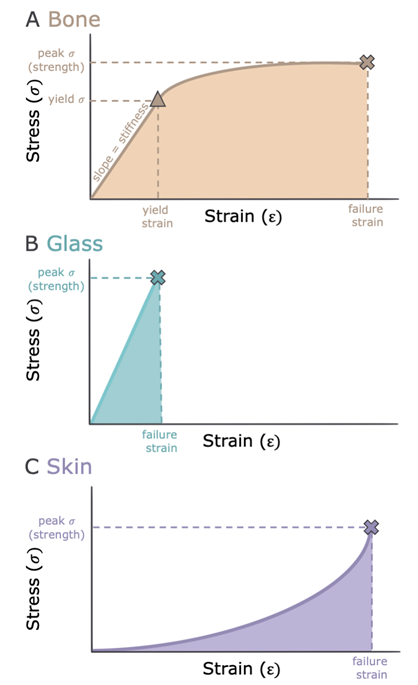
Figure 5.10—Stress-strain curves of bone (A), glass (B), and skin (C). Stress is a metric for material strength, and strain is a metric for deformation. The X’s represent peak failure (fracture), and the triangle on the bone graph represents the yield point. Shaded areas under each curve represent material toughness.
Now if you want to think about what differences in these properties mean for the behavior of materials, let’s compare stress-strain curves for two different materials. Our sample in Figure 5.10A is a pretty good representation of the stress-strain curve for bone: You can see it has fairly high strength, large extensibility, and a high toughness. If we were to compare that to another type of material—glass, for example—we’d see that both materials have similar strength, but compared to bone, glass has higher stiffness (Figure 5.10B). This higher stiffness results in less work required to fracture, meaning that this material cannot absorb energy very well, thus making it brittle. That’s why it’s easier to produce a fracture in glass than it is in bone and why bone makes a better material for building skeletons than glass does!
Let’s take another look at our standard stress-strain curve. Rigid and many tensile materials—things like horn, bone, and keratin—have concave-down stress-strain curves, such as Figure 5.10A. This means that as the material nears its breaking point, it requires less and less stress to deform. Pliant materials, in contrast, usually have a concave-up or J-shaped stress-strain curve, such as Figure 5.10C. Thus, as pliant materials are deformed, it takes more and more stress to keep deforming them. But how do we get this J-shaped curve? J-shaped curves can be produced in materials if they have tensile fibers embedded in a more pliant matrix. As the material is stretched, fibers are aligned (as we see occurring in skin) and kinky fibers straighten out (as happens in arterial walls)—both of these changes increase the material’s resistance. This type of concave-up stress-strain relationship has some advantages:
- It offers built-in protection against breaking as the risk of breaking gets closer. For example, the pliant nature of our arteries is really valuable because it follows this rule and thereby helps prevent aneurysms (i.e., burst blood vessels).
- It also helps impede the spread of cracks through the material. J-shaped curves have less area under the curve compared to concave-down curves—this means that they absorb less energy. Energy release drives the spread of cracks through a material, which can ultimately cause a failure of the entire structure. So by absorbing less energy, pliant materials have less energy to release; this helps prevent cracks, which helps keep failures local (if they were to occur).
But why do we care about crack formation and mitigating it? Well, cracks are bad for materials, because they act as stress concentrators, meaning they focus the application of force on a very small area (specifically, the tip or sharp edge of the crack). This concentration results in an increase in the intensity of the force on a small area and thereby increases the stress on the material. If stress is increased beyond the material’s capacity, it can result in failure of the structure. Living organisms very much benefit from avoiding cracks in their materials, because cracks can lead to a major failure of structures; such structural failures can result in the organism’s death or at the very least remove an individual from the reproductive pool for a while, which is just about as bad as dying from an evolutionary fitness perspective. So it’s advantageous for organisms to avoid cracks or to be able to mitigate crack formation when they do form, and they do so in two major ways:
- Organisms mix pliant materials with rigid materials in composite structures. When cracks develop in composites, the cracks are prevented from spreading when they encounter pliant portions of the composite because pliant materials have that J-shaped curve and are really resistant to crack formation. For example, the pliant elastin in your skin (Figure 5.1B) prevents cuts from expanding.
- Organisms also have rounded cavities throughout rigid materials. When cracks spread and encounter these cavities, the stress that was concentrated at the tip of the crack is spread out along the wall of the cavity. By spreading the stress along the cavity wall, the area over which the force is applied increases, and therefore the stress is decreased. We can see an example of such rounded cavities when we look at the structure of compact bone in vertebrate bones (Figure 5.1C).
At this point, we’ve spent a lot of time on measuring the loads that materials encounter and how the type or structure of the material influences the way in which the load affects a structure. But why is this important? One major reason is that if structures cannot handle the loads they encounter, they’ll fail, and this could be very bad for the organism—again, either leading to death or taking it out of the reproductive pool for a while. So typically organismal structures are at least slightly “overdesigned”—in other words, they can withstand higher forces than they usually encounter. This degree of “overdesign” is called a safety factor, which is determined by taking the ratio failure load / usual load. This ratio should always be greater than one; otherwise, the structure will always be broken. Let’s consider bone again, as an example. If a bone breaks at a strength of 200 MegaPascals (MPa) but during running bone typically only experiences 50 MPa, then we could take the ratio 200 MPa / 50 MPa and it would show us that bone has a safety factor of 4. This means that bone is capable of withstanding loads up to four times greater than the typical maximum load experienced during normal activity. And the advantage of having high safety factors is that it confers the ability to withstand unexpected high loads! However, safety factors cannot be indefinitely high. There are limits to the degree of “overdesign” that the body can accommodate because it is expensive (energetically speaking) to build and carry around extra material. This is why we see differences in safety factors across organisms and even across the specific parts of an organism. For example, if we were to consider the bones of the mammalian leg, the femur has a higher safety factor than the bones of the lower leg (i.e., the tibia and fibula). This is because more material farther from the body costs more energy to move around, so extensive overbuilding of the tibia and fibula will result in a huge energetic expense every time we walk around.
Now, there are trade-offs when we consider mechanical properties, and this is because single materials usually cannot maximize all potentially advantageous biological properties. We can think of this as a bit of a “jack-of-all-trades, master of none” problem. So, for example, stiff materials aren’t great at absorbing energy, and strong materials tend to have limited extensibility. As a result, organisms tend to be composed of many different materials with different properties that correspond with the performance of different functions. Consider our own bodies: We have stiff bones to transmit forces, but our tendons, which are made of collagen, allow elastic energy storage and recoil during locomotion. What’s more, a single material can actually vary in its properties due to differences in components or organization, and these variations also often relate to differences in function. John Currey examined the mechanical properties of bone and found that bone (which we can think of as a pretty standard and invariable biological material) actually varies substantially across species. And this variation actually reflects differences in mechanical properties related to function. In his work, when Currey compared a deer antler to a cow femur (both of which are mammalian bones), he found that the antler absorbed more energy than the femur and as a result was better able to withstand impacts (Currey, 1970). This makes a certain degree of sense if you think about the role of an antler in deer ecology (often as a combat tool during territorial disputes) compared to the role of the femur in cows (to support body weight and for locomotion). Further, when he looked at the tympanic bullae of whales (part of the skull, near the ear), he found that whale tympanic bullae are stiffer than normal bone (i.e., a cow femur), thereby making the bullae more effective in transmitting sound waves to the middle ear bones. What this work demonstrates is that even the same material can show differences in its mechanical properties, depending on what structure it contributes to and the function of that structure.
Consequences of Environmental Factors
While there are many different aspects of the environment that can influence form-function relationships, one of the most influential aspects is the type of fluid that an animal is moving through. Fluids are materials that have no fixed shape and yield easily to external forces. By this definition, fluids include all gases and liquids. Bringing Newton’s third law back one more time for this section, even though fluids easily deform, they also exert an equal and opposite force back on the objects that are pushing on them.
The study of the consequences of how fluids impact motion is called fluid dynamics and is broken into two categories depending on whether the fluid surrounding the object is still, static fluids or moving, dynamic fluids.
For static fluids, the main forces acting on an animal are the pressure and buoyancy. Pressure is our metric for measuring forces applied in multiple directions. For terrestrial vertebrates, our main pressure is air pressure, which changes with weather conditions, temperature, and altitude. This is because air is a mixture of several different gases, including nitrogen, oxygen, and carbon dioxide. Each of these gases independently produces its own pressure, and the sum of all these pressures is what we call the total pressure. As the relative amounts of gases change, the partial pressures of each gas change, changing the total pressure. For example, as you drive up a mountain, the relative amount of oxygen present in the air decreases, which decreases the partial pressure of oxygen as well as the total air pressure. You’ve probably felt this as you feel the need to “pop” your ears to equalize the changing pressure inside your body compared to outside your body. A similar concept applies to aquatic vertebrates, but here the surrounding pressure is from the water pushing on the object, and typically, water pressure increases with increased depth.
An additional static metric that we need to consider in the aquatic environment is that of buoyancy, or the force exerted by a fluid that opposes the weight of an object. Buoyancy is closely tied to the relative density of the object relative to the density of the fluid that an object is moving in. If the density of the object is less than the density of the fluid, then the object will float. If an object has a greater density than the surrounding fluid, it will sink. For fully aquatic vertebrates, the most energetically efficient strategy for moving through a static fluid is to be neutrally buoyant, meaning that the density of the organism is equal to the density of the surrounding fluid. Many aquatic vertebrates have specialized structures, such as the swim bladder of teleost fishes or the oily liver of sharks, that enable them to adjust and maintain neutral buoyancy as they move through water of different depths.
5.4 Form-Function Relationships in the Real World
In this section we are going to apply the concepts covered above in two areas of biomechanics: locomotion and feeding. We have incorporated the discussion of the ecological and evolutionary implications of these types of form-function relationships.
Locomotion
The way a vertebrate moves, its locomotion, is dependent on the environments in which it must move through. The three main types of locomotion include terrestrial locomotion, or methods of moving on land; aquatic locomotion, or moving through water; and aerial locomotion, also known as flying.
Fluid Locomotion
Both aquatic and aerial methods of locomotion are dependent on an organism’s ability to push against the fluid they are trying to move through.
One way this can be accomplished is by using drag-based locomotion. A force that acts in an opposing parallel direction to the motion of a moving object with respect to the surrounding fluid is called drag (Figure 5.8). So, for example, if a fish is trying to swim upstream, then the drag is the force that is working against the fish’s aquatic locomotion. If we dive a little deeper (pun intended), then we can look at why so many aquatic organisms have a similar body form. There are two major components to drag. Friction drag is the resistance of a fluid moving over the surface of an object. Meaning that as a fish is swimming through water or a bird is flying through air, the fluid that is directly touching the moving organism will be slowing down the longer it interacts with the surface of the organism (Figure 5.8). Now remember Newton’s third law, for every action there is an equal and opposite reaction. Thus, the fluid is also applying a force to the fish or bird trying to swim or fly. If an animal that moves through a fluid wants to decrease friction drag, then they would need to decrease their surface area. The second component of drag is pressure drag, or the resistance an object incurs as it moves itself through a fluid (Figure 5.11). In order to minimize pressure drag, organisms need to minimize the size of the parts of their bodies that hit the fluid first. This is why we see many aquatic and aerial animals that have a lemon-shaped, or fusiform, body shape. Anatomists are using what they know about these two components of drag along with experimental studies to explore better ways to design underwater vehicles (i.e., Wainwright and Lauder, 2020). This intersection of biology and engineering is called biomechanics or bioinspired design.
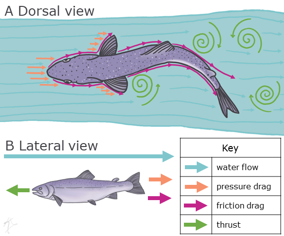
Figure 5.11—Drag-based locomotion from the dorsal view (A) and lateral view (B). Arrows show the vectors of different forces acting in drag-based locomotion, with blue arrows representing water flow, orange arrows representing pressure drag, pink arrows representing friction drag, and green arrows representing thrust.
In order to propel themselves forward in a fluid environment, organisms must produce a force in the opposite direction of drag; this force is known as thrust (Figure 5.11). We can tell quite a lot about how an organism produces thrust by looking at their body shape. The thrust-producing parts of aquatic animals will aim to reduce drag while maximizing thrust. So, for example, when you think of a fish (Figure 5.11), they use their deep (tall) bodies and caudal fins to produce thrust in a side-to-side direction, but otherwise they are fairly thin to minimize drag. Whereas most fishes swim by moving their bodies side to side, marine mammals, like whales and dolphins, have tails that are rotated 90 degrees compared to the fishes. This means that instead of pushing on the water by moving side to side, or laterally, these vertebrates will produce thrust by moving their bodies up and down, or dorsoventrally. This difference reflects the constraints placed on animal form based on evolutionary history. The ancestors of marine mammals were terrestrial and had limbs. Therefore, their ability to swim is constrained by the anatomy they started with from their terrestrial ancestors. We can actually measure the amount of thrust an organism produces using a method called digital particle image velocimetry (DPIV) developed by Willert and Gharib (1991). To use this method, researchers use high-speed video cameras and neutrally buoyant particles to measure the velocity of the fluid that an animal moves. Bringing Newton’s third law back again, by measuring how fast the fluid around the animal is moving, we can calculate how much thrust the animal is using to push that fluid in order to achieve locomotion.
The other form of fluid locomotion is lift-based locomotion. When force is perpendicular to the oncoming flow direction, we call this force lift. By angling the leading edge of the wing or fin, the edge that hits oncoming flow first, swimming and flying animals can control how much fluid is flowing above versus below the limb (Figure 5.12). As an animal flaps its wing or fin, it changes the angle of the leading edge (the edge that interacts with oncoming flow first) so that there is always a positive, lifting pressure below the limb that pushes the animal in the opposite direction of gravity and perpendicular to oncoming flow.
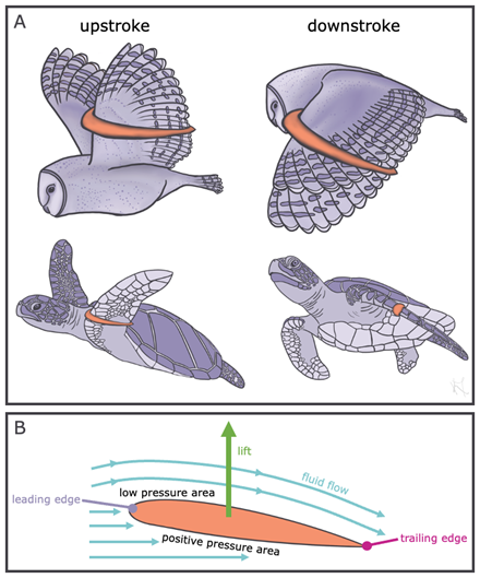
Figure 5.12—Lift-based locomotion. Examples of animals using lift-based locomotion (A) show how the angle of the limb changes during the upstroke and downstroke in an owl and sea turtle. The orange shape represents the limb cross section and highlights how the limb angle changes. A schematic of the limb cross section (B) shows how the fluid flowing around the limb provides positive pressure areas under the limb and low-pressure areas above the limb, generating lift perpendicular to fluid flow.
Terrestrial Locomotion
When vertebrates moved from the aquatic to the terrestrial environment, the forces required for locomotion shifted. As seen in the previous section, in the aquatic environment, animals primarily rely on thrust and lift-based locomotion. On land, instead of pushing against the surrounding fluid, locomotion requires that animals push off the ground, and the reacting force propels the animal forward. We call this force the ground reaction force (GRF), and the resting GRF, when the animal is not moving, is the weight of the animal.
As vertebrates moved onto land, they benefited from lower viscosity than moving through water but also lost their buoyancy to counteract gravity. So terrestrial vertebrates needed adaptations to their bones, muscles, and postures to move effectively on land. As the force of gravity became a larger factor in locomotion, vertebrate limbs moved more ventrally to what is called a sprawling posture (Figure 5.13). Early vertebrates and modern amphibians who use this sprawling posture rely on lateral motions, similar to how fish swim. What is different is that instead of pushing off the fluid with lateral undulations, vertebrates with sprawling postures use the opposite arm and opposite leg to produce GRFs that propel them forward. As vertebrates became more terrestrial, many taxa furthered this pattern by moving their limbs underneath their body in an upright posture (Figure 5.13). Upright postures allow animals to produce more efficient GRFs, because forces are applied directly through the limb rather than laterally, enabling faster locomotor speeds.

Figure 5.13—Sprawling versus upright posture. Model diagrams are provided for each posture as well as an alligator and human example. All models show the axial skeleton in tan, the pectoral/pelvic girdles in purple, the upper limb bones in pink, and the lower limb bones in blue.
As vertebrates became more specialized for living in different terrestrial environments, we began to see additional locomotor specializations. For example, vertebrates that use arboreal locomotion tend to have longer forelimbs with extra surfaces for improving gripping, while animals that specialize in jumping, or saltatory locomotion, tend to have the opposite body proportions, with longer hindlimbs and proportionally shorter forelimbs.
Human Locomotion
Of course, humans fall into this broad category of “organisms” we’ve been talking about here, and it should come as no surprise that locomotion is important for us too. Movement is essential for individual psychological and physical well-being. In fact, regular physical activity helps prevent a whole host of diseases, including things like heart disease, cancer, osteoporosis, and diabetes, among others. Furthermore, it helps with the prevention and management of psychological disorders like depression, anxiety, and others. And yet less than half of the world’s population has sufficient activity levels to maintain their physical and mental health (that’s 4 billion people who aren’t moving around enough!).
By integrating our understanding of anatomical structures and the physical principles that govern movement, we can gain a more complete understanding of human locomotion and apply that understanding to the development of new tools, technologies, and training to help improve mobility, physical activity, and ultimately human health. This is a primary focus of the fields of human biomechanics and kinesiology. In these disciplines, anatomic and physical principles can be employed in the study of human locomotor disorders, such as those observed in individuals with cerebral palsy, and outcomes of this work can inform health-care decisions related to surgical and other types of medical interventions intended to improve a person’s locomotor ability and quality of life. Indeed, the impacts of this type of research go beyond just the scientific realm: It is used for athletic training and equipment development, by the film and gaming industry in the production of realistic CGI, by engineers and manufacturers for the development of ergonomic tools and furniture, and in medicine in novel approaches to joint surgery and the engineering of powered exoskeletons for people with paralysis.
Box 5.2—When Form Doesn’t Match Function
Earlier in this chapter, we talked about how the vertebrate skeleton can be thought of as a collection of levers. In many cases, such as the example in Figure 5.8, the function that an animal uses matches the lever system that is observed in their skeleton. In Figure 5.14A, we have the forelimb of several different vertebrates as well as their main method of locomotion. For each of these limbs, we’ve color coded the parts of the limb that represent the lever system for forelimb extension (a.k.a. what happens when the triceps muscle flexes). Some of these forelimb levers are built for strength, such as the diggers noted in the figure, while other forelimb levers are built for speed, such as runners. Now let’s look at the sloth forelimb in Figure 5.14B. Sloths are relatively slow creatures that spend most of their time with their forelimbs extended hanging from the branches of trees. Look at their limb structure and think through the following questions:
- Is the sloth forelimb built for strength or for speed based on the lengths of the lever arms?
- What evolutionary advantage would being fast or strong have for the sloth?
- If there is no strong evolutionary selection for being fast or strong, what happens to the anatomy of the skeletal system?

Figure 5.14—When form doesn’t match function. The forelimbs of several vertebrates are provided (A) to compare with the sloth (B). Each limb is color coded to show the fulcrum (orange), in-lever (pink), and out-lever (blue) for forearm extension. Under each limb, the animal and its primary mode of limb movements are provided.
Feeding
Feeding can be broken down into three major categories: searching, acquisition, and ingestion. You will learn more about how animals sense their environment in later chapters, and you have learned how animals move in the previous section of this chapter, so here we will focus on food ingestion. The anatomy a vertebrate has and the environment in which it lives can tell us a lot about how an animal ingests their food without ever needing to see them feeding in action. In terrestrial vertebrates, looking at skull and tooth shape can tell us if a vertebrate is likely going to have a primarily herbivorous, carnivorous, or omnivorous diet. Skull shape will tell us where muscles meant for chewing attach, with larger attachment sites relating to relatively more/stronger muscles. Tooth shape can tell us if a tooth is meant for grinding (e.g., molars) or slicing (e.g., incisors, canines). You will learn more about tooth shape when we discuss the skull in Chapter 8, so for now we will focus more on function than on the specific names of the different types of teeth. Herbivores, who have a mostly plant-based diet, have more grinding teeth, fewer slicing teeth, and muscles that allow for side-to-side movements for grinding of plant materials (Figure 5.15). Carnivores, who rely mainly on eating meat, have more teeth meant for slicing and have more muscles for stronger bite forces (Figure 5.15). Omnivores, such as humans, who eat a combination of plant and animal diets, have more generalized tooth structures and muscles meant for both slicing and grinding (Figure 5.15).
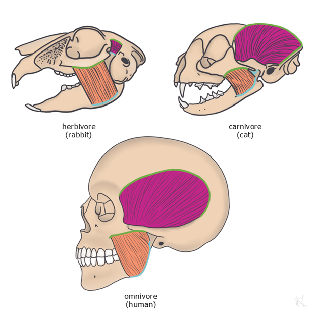
Figure 5.15—Feeding morphology in an herbivore (rabbit), carnivore (cat), and omnivore (human). The chewing muscles are color coded to show the importance of bite force from the temporalis muscle (pink) compared to the importance of grinding from the masseter muscle (orange). For both muscles, the areas of attachment for each muscle’s origin (green) and insertion (blue) are outlined.
Box 5.3—Try It Yourself! Using Open-Source Platforms to Measure Form-Function Relationships
In addition to observing the form-function relationships in the real world, many repositories and software programs have been developed over the past 20 years to aid in the collection of digital morphological data.
There are several repositories where you can download scans of specimens. One such repository is MorphoSource.org (Boyer et al., 2016). Funded by the National Science Foundation, MorphoSource allows users to share and download anatomical images, such as computed tomography (CT) scans, models, magnetic resonance imaging (MRI) scans, photogrammetry, and more. MorphoSource accounts are free, but often you will need to request permission from the data owner in order to download or use the files of interest. This allows museums and other institutions to keep track of how the data are being used.
After you’ve found a digital specimen or specimens you want to collect measurements on, there are also free, open-source software tools to allow you to collect data without expensive software packages. One example is 3D Slicer (Fedorov et al., 2012), which is used heavily in the medical industry for quantifying and modeling anatomy from medical images (CT and MRI). There are many plugins for 3D Slicer; one that is particularly useful for measuring anatomical structures is SlicerMorph (Rolfe et al., 2021). The developers of SlicerMorph have a repository of tutorials if you’d like to test out these tools yourself, which can be found at https://github.com/SlicerMorph/Tutorials.
5.5 Further Reading
- Alexander, R. McNeill. Principles of Animal Locomotion. Princeton: Princeton University Press, 2003.
- Irschick, Duncan J., and Timothy E. Higham. Animal Athletes: An Ecological and Evolutionary Approach. Oxford: Oxford University Press, 2016.
- Vogel, Steven. Comparative Biomechanics: Life’s Physical World. Princeton: Princeton University Press, 2013.
5.6 References
- Alexander, R. McNeill. Principles of Animal Locomotion. Princeton: Princeton University Press, 2003.
- Boyer, Doug M., Gregg F. Gunnell, Seth Kaufman, and Timothy M. McGeary. “Morphosource: Archiving and sharing 3-D digital specimen data.” The Paleontological Society Papers 22 (2016): 157–181.
- Currey, John D. “The mechanical properties of bone.” Clinical Orthopaedics and Related Research 73 (1970): 210–223.
- Fedorov, Andriy, Reinhard Beichel, Jayashree Kalpathy-Cramer, Julien Finet, Jean-Christophe Fillion-Robin, Sonia Pujol, Christian Bauer, Dominique Jennings, Fiona Fennessy, Milan Sonka, et al. “3D Slicer as an image computing platform for the Quantitative Imaging Network.” Magnetic Resonance Imaging 30 (2012): 1323–1341.
- Haldane, J. B. S. Possible Worlds and Other Essays. London: Chatto & Windus, 1927.
- Irschick, Duncan J., and Timothy E. Higham. Animal Athletes: An Ecological and Evolutionary Approach. Oxford: Oxford University Press, 2016.
- LaBarbera, Michael. It’s Alive! The Science of B-Movie Monsters. Chicago: University of Chicago Press, 2013.
- Rolfe, Sara, Steve Pieper, Arthur Porto, Kelly Diamond, Julie Winchester, Shan Shan, Henry Kirveslahti, Doug Boyer, Adam Summers, and A. Murat Maga. “SlicerMorph: An open and extensible platform to retrieve, visualize and analyze 3D morphology.” Methods in Ecology and Evolution 12 (2021): 1816–1825.
- Vogel, Steven. Comparative Biomechanics: Life’s Physical World. Princeton: Princeton University Press, 2013.
- Wainwright, Dylan K., and George V. Lauder. “Tunas as a high-performance fish latform for inspiring the next generation of autonomous underwater vehicles.” Bioinspiration & Biomimetics 15 (2020): 035007.
- Willert C. E., and M. Gharib. “Digital particle image velocimetry.” Experiments in Fluids 10 (1991): 181–193.
