
7 Yield Curve
“Yo word is yo bond,” which in today’s Hip Hop Culture has become word is born.
Geneva Smitherman
7.1 Bond Basics
It is January 1, 2030. You give XYZ Inc. $1,000 today, and they promise to pay you back in two years. Congratulations, you just bought a bond!
The $1,000 is called the face or par value, and the maturity date is two years from now, January 1, 2032 (when you get the face value back). Not surprisingly, you own a two-year bond.
Of course, you must be compensated for the time value of money—$1,000 two years from now is worth less than $1,000 right now. So XYZ also promises to pay you interest at regular intervals—say, every six months. The coupon rate, say 5%, tells you the interest you will be paid in a year. Five percent of $1,000 is $50, so you will get two payments of $25.
Because the coupon (interest) and final payments are on a strict schedule, bonds are called fixed-income securities. Bonds are debt, and they give investors a safer but lower return, on average, than stocks which are equity (since they involve ownership of a corporation).
The jargon—special words or technical language used by professionals—can make financial products and choices difficult to understand. We can make your bond come to life with Excel. As you enter the information, think about the trade-off involved here—the lender (you) gives up money now in return for future payments from the borrower (XYZ). This is the core idea.
STEP Open a blank Excel workbook and save it as YieldCurve.xlsx. In cells A1 to A5, enter the dates 1/1/2030, 7/1/2030, 1/1/2031, 7/1/2031, and 1/1/2032, respectively. In cell B1, enter -$1000; this is the amount you invested in the bond (hence the minus sign). Cells B2, B3, and B4 represent the coupon payments, so enter 25 for each of those cells. At the end, you get the last interest payment plus the face value back, so cell B5 is 1,025.
Your spreadsheet now looks quite familiar, given the work we did on present value and the internal rate of return (IRR). That’s right; a bond is just another application of those ideas. You start with a negative number that represents your investment, then get a stream of income over time that is your return on investment.
The IRR is a measure of the quality of an investment; the bigger it is, the better the investment. We can compute the IRR for these cash flows at these dates using Excel’s XIRR function. It incorporates the dates at which the flows are paid and received and returns the annualized internal rate of return.
STEP Enter the formula =XIRR(B1:B5,A1:A5) in cell C1 and format it as a % with two decimal places. In cell D1, enter the label IRR = YTM so that your spreadsheet replicates Figure 7.1.
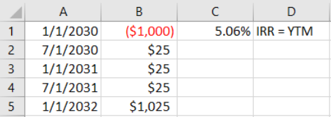
The IRR is a little over 5% because you received the annual interest payment of $50 a little ahead of time: $25 halfway through the year and another $25 at the end of the year instead of all $50 at the end of the year.
STEP Confirm this by changing cells B2 and B4 to 0, cell B3 to $50, and cell B5 to $1,050.
Cell C1 now shows the IRR as 5.00%. This shows that the XIRR function is working as advertised. It also shows that the timing of the coupon payments is critical. Your spreadsheet is now displaying a different bond than the one in Figure 7.1. The IRR of the bond in Figure 7.1 is higher than the one on your spreadsheet because of the timing of the interest payments.
The IRR for a bond is called the yield to maturity (YTM). It is calculated as if the investor will hold the bond until the maturity date. But they might not. Bonds can be traded before they mature in the secondary market.
A zero-coupon bond, also called a strip, is just what it says—it has no interest payments.
STEP Change the value in cell B3 to 0 (so the values in cells B2, B3, and B4 are all 0), and make cell B5 $1,000.
The YTM is now zero. That’s terrible. No investor would buy this bond. To entice buyers, the issuer must sell the bond at a discount (or below par).
STEP Change cell B1 to –$900.
That’s better. Now the YTM is about 5.4%. Investors are compensated for lending $900 today by getting the face value of the bond, $1000, in two years. Someone might be willing to buy this bond and lend the issuer $900.
Bonds are complex financial assets. They have many variations, and the jargon is intimidating, but no matter how complicated it gets, the idea is that a bond is a promise—money in the future is promised in return for money now.
Yield Data
With a basic understanding of a bond and how it works, we can get yield data and create visualizations, including that of our ultimate goal: the yield curve over time.
We will work with US Treasury securities with different maturity dates. They all work like bonds, but they have different names depending on their maturity dates: Treasury bills mature in 1 year or less, Treasury notes in two to 10 years, and Treasury bonds in 20 or 30 years.
First, we will examine a single security over time, but our eventual goal is to visualize a richer dataset with yields for different maturities over time. This will give us the yield curve.
STEP Insert a sheet in your workbook, rename it GS1, and enter the Series ID GS1 (for government security maturing in 1 year) in cell A1. Use the FRED Excel add-in to get the data. Use FRED’s charting tools to make a chart with recession shading, like Figure 7.2 (made in October 2023). Refer back to the work we did using FRED to get unemployment data (in chapter 5) if needed.
Figure 7.2 shows the yield on a one-year US Treasury bill on a monthly frequency from April 1953 to September 2023. Your spreadsheet will have this series up to the previous month in which you created it.
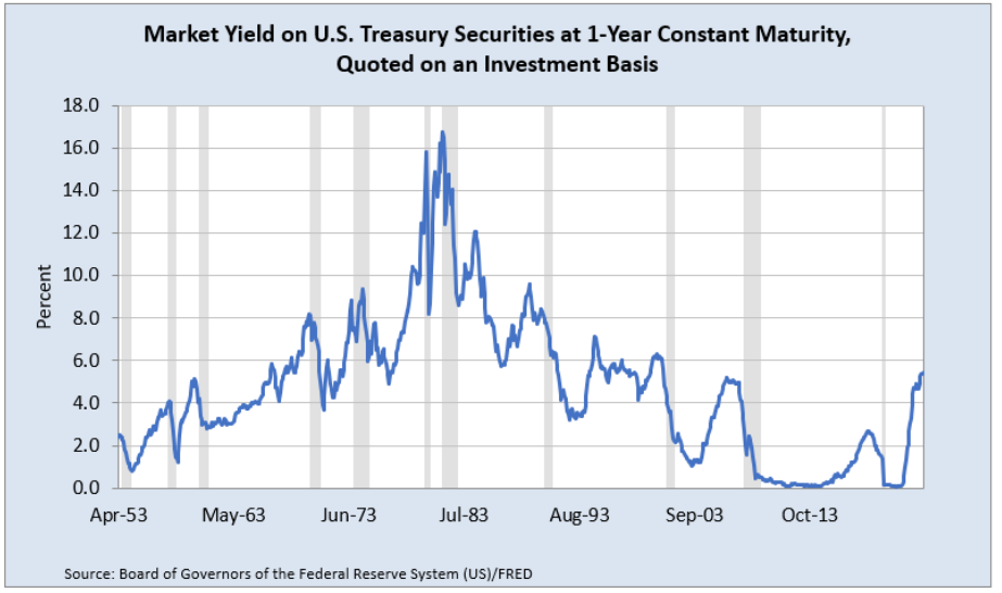
Source: Board of Governors of the Federal Reserve System (US) via FRED, Public Domain Data / FRED Terms.
Unlike the unemployment rate, which rose in every recession, one-year US Treasury bill yields are mostly falling when they enter the shaded bars. This is because the government is actively trying to use monetary policy to lower interest rates to stimulate the economy.
The US Federal Reserve (Fed) acts as a central bank and influences many different interest rates, including bond yields, by controlling the federal funds rate (the interest rate at which banks lend reserves to each other).
The key point for our yield data is that one-year US Treasury bill yields are not directly controlled by the Fed. They are the outcome of supply and demand. Bonds, including US Treasury securities, can be traded before their maturity dates. It is the bond market that determines yields.
It is easy to see in Figure 7.2 that in the early 1980s, yields were very high, in double-digit territory. Why? Certainly, a contributing factor was high inflation at that time. The yield had to be high to entice the lender to part with money now to be paid back later.
STEP Return to your bond demonstration sheet. You should see the zero-coupon bond. You part with $900 now and get $1,000 in two years, which has a YTM of about 5.4%.
In the early 1980s, there would be no way you would give anyone (XYZ or the US government) $900 in return for $1,000 in two years. The $1,000 you got back two years later would be so watered down by the high inflation at that time that you would refuse that deal. So the issuer would need to raise the yield by lowering (discounting) the bond by more than $100.
STEP Change cell B1 to –$800. What happens?
Not surprisingly, the YTM increases to almost 12%. Is that enough to get you to make the trade? Not in August 1981.
STEP Return to the GS1 sheet. Enter the formula =MAX(B:B) in cell C8 to see the highest yield in the dataset. Scroll down to find when it occurred.
In August 1981, the market, or equilibrium, yield was 16.7%. You would not lend unless you got that yield, just like you would not buy apples from a particular seller if their price was higher than the market price that many other sellers were selling apples for.
STEP Return to the sheet with the simple two-year bond we were playing with and use Solver to find the discount in the bond price needed to produce a yield of 16.7%. Be sure to uncheck (if needed) Solver’s Make unconstrained variables nonnegative option, since we want a negative number in cell B1.
You should find that the bond price is roughly $734, so it is a discount of $266 from the par value.
The inverse relationship between the yield and the bond price is a fundamental concept in the bond world. The Excel implementation of a bond makes it easy to see: The lower the price (the bigger the discount) in cell B1, the higher the yield.
Yields for Different Maturities
Just like GS1, the yield on a 1-year US Treasury bill, FRED has data for yields on US Treasury securities with different maturities, also known as the term structure. We will get data on US Treasuries from 3-month to 30-year terms.
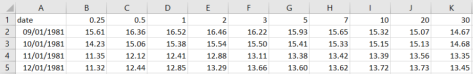
STEP Insert a sheet in your workbook and name it TermStructure. In individual cells in the top row, enter the following Series IDs: GS3M, GS6M, GS1, GS2, GS3. GS5, GS7, GS10, GS20, and GS30. The M stands for months, and the numbers indicate the length of time. So GS6M is a 6-month US Treasury bill, and GS20 is a 20-year Treasury bond. Click the Get FRED Data button.
The series start at different dates. We need to find the latest date and start them all from that point so that we can see how the yields varied by maturity on the same date.
STEP The latest starting date in row 8 is 9/1/1981. Copy this cell and paste it in cells E4, G4, and so on until S4. Update the data.
Each row has yields for differing maturities of US Treasury securities for a particular point in time. Thus, each row has the data for the yield curve for that month.
Here is how the Fed describes the yield curve:
Investors can trade Treasury securities freely between issuance and maturity. As the market price of Treasury securities varies over time, so does their implied yield—their return relative to their price. At any given time, there is a wide range of Treasury securities with different maturities outstanding. Market forces tend to ensure that the yields on securities with similar maturities are not dramatically different from each other. This feature makes it possible to summarize the information contained in the cross section of market-implied yields by a smooth curve of yield as a function of maturity—the yield curve.[1]
Thus, the yield curve shows yield by maturity. Let’s make one.
STEP Copy the TermStructure sheet and rename it YieldCurve. Change each of the value labels in row 7 to the corresponding length of time in years. Cell B7 is 0.25 (you may have to increase the decimal places displayed), cell D7 is 0.5, cell F7 is 1, and so on. Delete rows 1 to 6. Delete the date columns, starting with column C (so C, E, G, and so forth, all the way to S). Finally, select the yield data (from B2 to the last row in column K) and display two decimal places.
You now have a dataset that looks like Figure 7.3. It has dates in column A, lengths of maturity in years in row 1, and yields for each month by maturity. These are the inputs needed to make a yield curve.
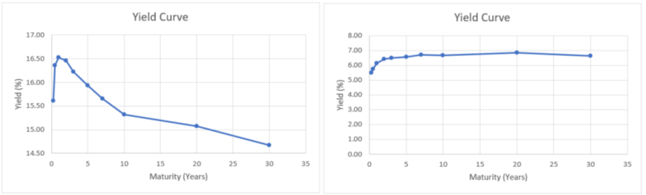
STEP Select cells A1:K2 and insert a Scatter with Straight Lines and Markers chart. Add a title, Yield Curve, and label the axes Yield (%) and Maturity (years).
You just made your first yield curve. It is not common. Usually, it is upward sloping. The longer the maturity, the higher the yield, because lenders have to be rewarded for locking up their money for longer periods of time.
The 1980s were certainly exceptional economic times. The yield curve was inverted because yields for shorter maturities were higher than those for longer maturities. This usually means bad tidings for the economy.
There is another step we could take to make our yield curve a true curve: We could fit a smooth curve to the data. The smoothed curve version of yield as a function of maturity is what most people call a yield curve. There are many ways to fit such a curve, and it gets complicated, so we will stay with our rudimentary version that connects the data with straight lines.
We can easily make another yield curve so we can understand what the yield curve is telling us. We work smart by using the edit SERIES formula approach.
STEP Copy and paste the chart. Click on the data and edit the SERIES formula by changing the 2 to 222 in the y-axis part of the formula, YieldCurve!$B$222:$K$222.
You just produced a yield curve for January 2000. Unlike September 1981, it rises fast, then stretches out. Figure 7.4 compares the two yield curves.
While the slightly lower yield for 30 versus 20 years is unexpected, the January 2000 yield curve (on the right) is a typical yield curve. As the yield to maturity rises from very short term (starting at 30 days) to 2 years, yields rise quickly, but then they rise much more slowly as maturity increases.
We learned about bonds and yields, got yield data, and created yield curve charts. Next up, we work on fancier visualizations of yield curve data.
Takeaways
In everyday English, a bond is a connection between people (a bond of friendship) or objects (to bond is to glue things together). In finance, the connection is between lender and borrower.
A bond is a security in which a borrower (e.g., a firm or government) promises to pay back the face value at the maturity date and make interest payments at specific dates (to compensate the lender for the time value of money).
Unlike the two-year bond we implemented in Excel, most bonds are on a 30/360 calendar and have a high threshold of legalese, like this example:
(1) Interest. Ventas Realty, Limited Partnership (the “Issuer”) promises to pay interest on the principal amount of this Note at 4.125% per annum from July 16, 2015 until maturity. The Issuer will pay interest semi-annually in arrears on January 15 and July 15 of each year, or if any such day is not a Business Day, on the next succeeding Business Day (each, an “Interest Payment Date”). Interest on the Notes will accrue from the most recent date to which interest has been paid or, if no interest has been paid, from July 16, 2015; provided, that if there is no existing Default in the payment of interest, and if this Note is authenticated between a record date referred to on the face hereof and the next succeeding Interest Payment Date, interest shall accrue from such next succeeding Interest Payment Date; provided, further, that the first Interest Payment Date shall be January 15, 2016. The Issuer will pay interest (including post-petition interest in any proceeding under any Bankruptcy Law) on overdue principal and premium, if any, from time to time on demand at a rate that is 1% per annum in excess of the rate then in effect; the Issuer will pay interest (including post-petition interest in any proceeding under any Bankruptcy Law) on overdue installments of interest (without regard to any applicable grace periods) from time to time on demand at the same rate to the extent lawful. Interest will be computed on the basis of a 360-day year of twelve 30-day months.[2]
A bond is a way for borrowers to raise money. Firms often use bonds to fund operations, while government bonds pay for deficit spending (when outlays are greater than tax revenues).
The funds raised by issuing bonds are debt because the issuer has to pay the lenders back, just like they would pay back a bank loan.
The jargon in the bond world is intense. Knowing things like the difference between the coupon rate and the yield to maturity is critical for those who live in the bond world.
It is important to understand that the contract is ironclad, so the coupon rate and promised cash flows do not change as interest rates change. You might buy a bond in the secondary market above or below par value, so the spot rate (the IRR at the time you buy the bond) does change.
Higher interest rates produce lower bond prices. This fundamental law of bonds is easiest to see in a strip because there are no interest payments. The bond price will always be lower than the face value, but as the bond price (the amount you pay to buy the bond) gets farther from the face value (the amount you get at maturity), the higher the yield: “The U.S. Treasury yield curve is of tremendous importance both in concept and in practice. From a conceptual perspective, the yield curve determines the value that investors place today on nominal payments at all future dates—a fundamental determinant of almost all asset prices and economic decisions” (Gürkaynak et al., 2006, p. 1).
References
The epigraph is from p. 8 of Geneva Smitherman’s Black Talk: Words and Phrases from the Hood to the Amen Corner, Houghton Mifflin (1994). Here is the full entry for word is born!:
“An affirmative response to statement or action. Also, Word!, Word up!, Word to the mother! A resurfacing of an old, familiar saying in the Black Oral Tradition, “Yo word is yo bond,” which was popularized by the five percent nation in its early years. Word is born! reaffirms strong belief in the power of the word, and thus the value of verbal commitment. One’s word is the guarantee, the warranty, the bond, that whatever was promised will actually occur. Born is the result of the AAE [African American English] pronunciation of “bond”; see Introduction.”
Board of Governors of the Federal Reserve System (US), Market Yield on U.S. Treasury Securities at 1-Year Constant Maturity, Quoted on an Investment Basis [GS1], retrieved from FRED, Federal Reserve Bank of St. Louis; https://fred.stlouisfed.org/series/GS1.
The yield data in FRED are produced by the Fed, and it is a complicated process. A good source for digging into the details is Refet S. Gürkaynak, Brian Sack, and Jonathan H. Wright (2006) “The U.S. Treasury Yield Curve: 1961 to the Present,” Finance and Economics Discussion Series, Divisions of Research & Statistics and Monetary Affairs, Federal Reserve Board, Washington, DC.
7.2 Yield Curve Visualizations
We begin our visualizations of the yield curve with a clever way to easily control which month-year yield curve to display. Our strategy will be to use a Combo Box form control to enable the user to select a date. The selected month-year will be connected to a cell in the sheet, which we will use to get the yields via the OFFSET function. Finally, we will tie the chart to the selected yields by directly editing the SERIES formula. This will all make more sense as we actually do it.
STEP With yield curve data in columns B through K, dates in column A, and labels in row 1, click the Developer tab, then the Insert group, and select the Combo Box form control as shown in Figure 7.5. Click on the spreadsheet under your yield curve chart, and drag to place the control on the sheet. Right-click the control and choose Format Control. For the Input range, select from cell A2 to the last row with data in column A. For the cell link, select cell M1.
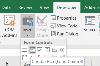
Source: Screenshot of Excel interface, © Microsoft Corporation.
It does not look like we have done anything, but we have. Our Combo Box is loaded with the dates in column A.
STEP Click on any cell in the sheet so that the Combo Box is not selected and then click the Combo Box control. Select any date.
Cell M1 now shows the row number of the date you selected. Next, we get the yield data for the chosen date.
STEP Enter the formula =OFFSET(A1,$M$1,0) in cell N1.
Excel displays the date for that row. The OFFSET function works by taking you to cell A1 and then going down however many rows are in cell M1 while staying in column A (that is what the zero says to do).
STEP Change cell M1 to 10. What happens?
Not only does the date in cell N1 change to the date in cell A10, but notice that the Combo Box control has also changed. Cell M1 is connected to the Combo Box, so you can use the Combo Box to set cell M1’s value or do the reverse and set the Combo Box’s value by entering a number in cell M1.
STEP Select cell N1 and fill it right to cell X1.
Now you are displaying the yields for each maturity for that month-year. This means all we have to do is edit the chart’s SERIES formula to display the yields in cells O1:X1.
STEP Click a point on the yield curve to see the SERIES formula in the formula bar. Remove the legend text and edit the y-axis so that the SERIES formula is =SERIES(,YieldCurve!$B$1:$K$1, YieldCurve!$O$1:$X$1,1).
We are ready to test our dynamic visualization of the yield curve.
STEP Click the Combo Box control and pick a date.
The chart immediately updates and shows you the yield curve for that date! The Combo Box control is an effective way to get user input.
STEP Use the Combo Box control to display yield curves from several dates. Try one from each decade. Definitely visualize the last row so you can see the current state of the yield curve.
If you play around a bit, you will see that the yield curve is usually upward sloping, but there are a variety of shapes. Inversion is when yields for longer maturities are lower than those for shorter maturities. This does happen, but it is not the usual shape of the yield curve. Before we discuss the interpretation of inversion, we will do some 3D visualizations.
3D Viz in Excel
What if we visualized all the month-year yield curves at once, in one chart? The yield would be the vertical axis in a 3D plot, with time and the maturities as the two horizontal axes.
STEP Delete the date text from cell A1 (the top-left corner of the data must be an empty cell). Select from cell A1 to the last row in column K. Click Insert and Recommended Charts and then select 3D Surface.
Excel puts a chart on your spreadsheet, but it certainly needs some cleaning up. What follows are the steps to produce Figure 7.6.
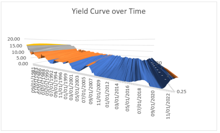
STEP Make the title Yield Curve over Time and delete the legend.
The problem with the chart on your screen is that the time axis (near the front) is long and the maturity axis is too narrow. This is because there are many more rows than columns. We need to widen the maturity axis.
STEP Right-click the surface and select 3-D Rotation. . . . Repeatedly click the up arrow in the Depth (% of base) setting until you start to see the maturity axis start to widen. You can go up to 2,000, so directly enter this value.
Your chart should now look like Figure 7.6. It still needs more work. The maturity axis labels are unclear, and too many dates are displayed. The vertical axis needs a label, and the way it is angled is not helpful. We will not bother trying to fix these issues because there is a big problem with Excel’s charting interface: Rotation is clumsy.
Excel provides X, Y, and Z rotation controls, and you can try them, but they are difficult to work with. We want to be able to easily spin the chart with the cursor. To do this, we will use Python.
3D Viz in Python
Python is “an interpreted, object-oriented, high-level programming language with dynamic semantics” (www.python.org/doc/essays/blurb/). That sounds complicated, but do not worry; Python is really easy to access and use. It is open-source (free), and its many users provide a strong support system.
As of this writing, generative AI (especially ChatGPT) can be used to write effective Python code.
Although you can download and install it on your personal device, we will use an even simpler approach, Google’s Colab environment.
STEP Click the link colab.research.google.com/ or enter it into your favorite browser. If needed, login to Google when prompted. Click on the Welcome to Colab link and read it.
The Colab notebook that you read is composed of executable and text cells. Across the top of the Colab screen are the usual menu items, and on the left is a table of contents with the sections in the notebook.
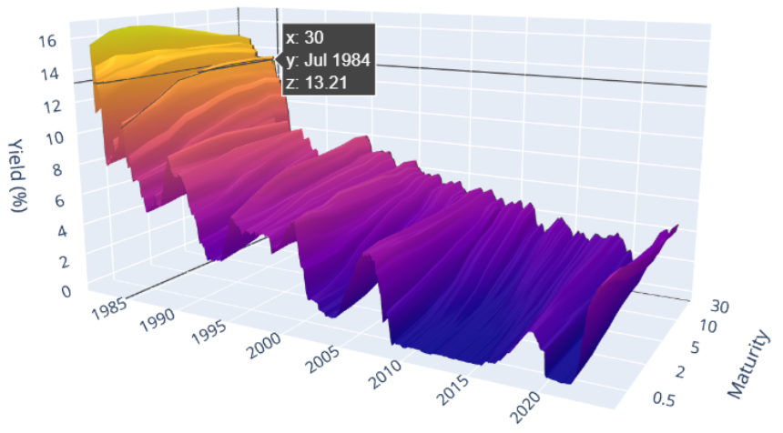
The yield data in the YieldCurve.xlsx workbook were uploaded to Google Drive. A few lines of Python code create a 3D plot that is easy to rotate and spin.
STEP Click the link dub.sh/3DVizYieldCurve or enter it into your favorite browser to see a Colab notebook that creates a 3D visualization of the data. Follow the instructions to spin the plot.
Figure 7.7 shows the Python visualization of the yield curve over time. Of course, the online version is live in the sense that you can spin it and use the cursor to get values at specific points on the surface.
Yield Curve Meaning
Our yield curve visualizations are certainly eye-catching, but what does the yield curve actually tell us? There are several ways to answer this question, but the most important use of the yield curve is as the market’s expectation of future economic performance.
Before we dig into how the yield curve can be used as a predictor, consider this: You follow a sports team that is expected to be really good this year, but they have aging stars at key positions. Then the betting odds of your team winning a championship would be higher for this season than a few years from now.
Conversely, if your team was bad now but had young players who could develop into superstars, their odds of winning in future years are higher than now.
You can stretch the time horizon even farther and think about odds a decade or longer from now. For so far into the future, all the teams would have similar odds (almost none of the current players would be active) unless there is some reason to believe that the ownership or management of a team is especially good or bad.
This thought exercise is quite similar to what the yield curve is doing. The yields are produced by supply and demand for each maturity. In a real sense, the yields for different maturities reflect the market participants’ overall outlook on the economy at different times in the future.
When the yield curve inverts and longer maturities have lower yields than shorter ones, it means that investors think yields and interest rates will be lower in the future. This is interpreted as pessimism because low interest rates are associated with the Fed trying to stimulate an economy in recession.
So is the yield curve any good at predicting the future?
STEP Return to your YieldCurve.xlsx workbook and insert a blank sheet. Use FRED’s Data Search tool to search for yield curve. Select the top 2 hits, T10Y2Y and T10Y2YM. Get the data and make separate charts with recession shading.
The daily chart is more jagged, but it tells the same story as the monthly frequency chart, shown in Figure 7.8. When the series dips below zero (so 2-year yields are higher than 10-year yields), the yield curve is inverted.
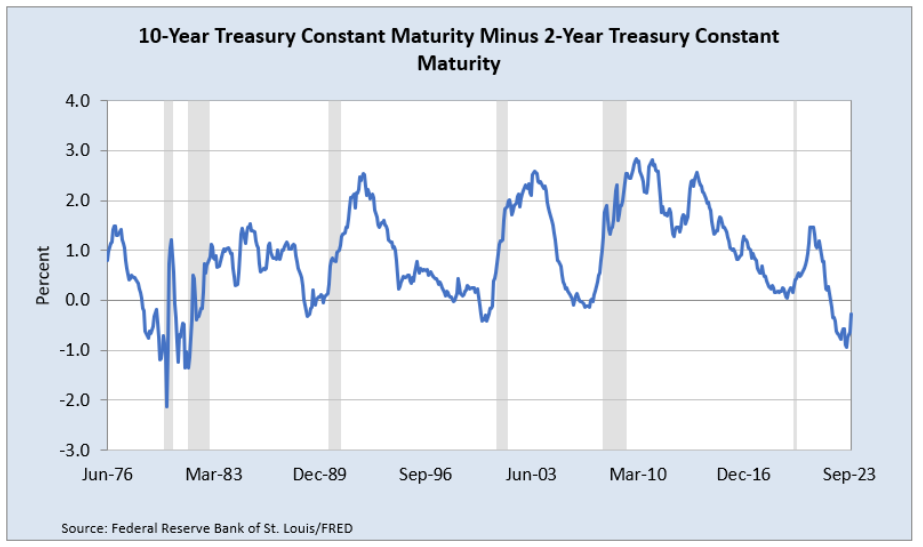
Source: Federal Reserve Bank of St. Louis via FRED, Copyrighted Data / FRED Terms.
Since 1969, an inverted yield curve has correctly predicted recessions shortly after the inversion (roughly within 15 months). Figure 7.8 shows that when the series goes below zero, a shaded bar soon follows—except the last one.
Is this time different? As of this writing, in 2024, the yield curve has been inverted for a record long time (www.google.com/search?q=yield+curve+record), yet the US economy seems strong. Will the yield curve be right again?
Takeaways
Excel can be used to make charts, and adding controls can make an Excel chart responsive to user input. We used a Combo Box control to allow the user to display the yield curve for a particular month-year.
Excel is not, however, strong data visualization software. In particular, its ability to manipulate charts, such as spinning a 3D plot, is quite limited.
Python, on the other hand, has extensive data display libraries. We used Google’s Colab environment to produce a 3D plot of the yield curve over time. It is simple to share the chart, and users can easily click and rotate it.
The yield curve itself has been the subject of extensive research. Analysts model the shape and fit curves to yield data.
Usually, there is a term premium for bonds with longer maturities. Investors have to be rewarded with higher yields when they lock up their money for longer periods of time.
One especially keen area of interest is the concept of an inverted yield curve.
Inversion occurs when long-term yields are lower than short-term yields (this is not common).
An inverted yield curve is strongly associated with a recession in the near future.
The yield curve, measured by 10-year minus 2-year YTM, inverted on July 11, 2023. It has remained inverted in the early part of 2024. There is great debate about whether this time it’s different.
References
For an overview of the yield curve with excellent graphics and an explanation of the meaning of the yield curve, see Bruce-Lockhart, C., Lewis, E., and Stubbington, T. “An Inverted Yield Curve: Why Investors Are Watching Closely.” Financial Times, April 6, 2022, ig.ft.com/the-yield-curve-explained/.
Federal Reserve Bank of St. Louis, 10-Year Treasury Constant Maturity Minus 2-Year Treasury Constant Maturity [T10Y2YM], retrieved from FRED, Federal Reserve Bank of St. Louis; https://fred.stlouisfed.org/series/T10Y2YM.
- Source: https://www.federalreserve.gov/data/nominal-yield-curve.htm ↵
- Source: EDGAR filing at the Securities and Exchange Commission website, www.sec.gov/Archives/edgar/data/740260/000110465915051467/a15-1495311ex4d2.htm ↵
