
2 Optimization with Solver
The first way of thinking that made the law about the behavior of light evident was discovered by Fermat in about 1650, and it is called the principle of least time, or Fermat’s principle. His idea is this: that out of all possible paths that it might take to get from one point to another, light takes the path which requires the shortest time.
Richard Feynman
2.1 The Lifeguard Problem
You are a lifeguard on a beach. You are standing on the shore; the water laps at your feet as the sun shines on your face. You timed yourself the other day, and you ran 100 meters in 20 seconds. You are much slower than the other lifeguards, but you are a superfast swimmer. You can swim 100 meters in 50 seconds—that’s only a few seconds off the freestyle world record! You like numbers, and a thought pops into your head: “It’s funny that I’m a slow runner and fast swimmer, yet I can still run 2.5 times faster than I swim—my run speed is 5 m/sec, while my swim speed is 2 m/sec.”
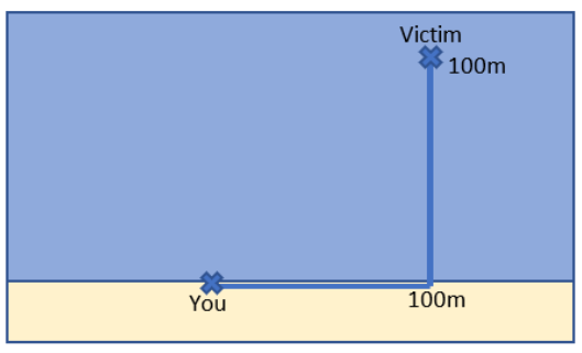
Suddenly, you see someone frantically waving in the water and hear cries of “Help!” They are exactly 100 meters to your right and 100 meters from the shore. Figure 2.1 shows the positioning. Your training kicks in, and you take off running along the shore toward the drowning person. Your goal is to get to them as quickly as you can. Your mind is consumed by a critical question: “When do I dive in and start swimming?”
Before we implement and solve this problem in Excel, let’s agree that you do have a decision to make. Consider these two paths:
(A) Based on the logic that you’re a faster runner than a swimmer, you could run 100 meters along the shoreline in 20 seconds and then swim 100 meters in 50 seconds, and you would reach the drowning person in 70 seconds. This path is the shortest swimming distance.
(B) On the other hand, you could argue that it is better to just dive into the water and make a beeline for the victim because this is the shortest total distance. The Pythagorean Theorem says that the hypotenuse is about 141 meters (sqrt(1002 + 1002)). This distance is much shorter than the 200 meters total distance required by running 100 and swimming 100 meters.
The problem, however, is to minimize not swimming distance or total distance but time—you have to get to the drowning victim as soon as possible. We know Path A takes 70 seconds, but what about Path B?
Path B takes a little longer than A. Here is the algebra involved in the computation:
[latex]t i m e = \frac{d i s t a n c e}{s p e e d} = \frac{141 m}{2 \frac{m}{s e c}} = 70.5 \text{seconds}[/latex]
Thus, running 100 meters and swimming 100 meters is better than swimming about 141 meters because 70 seconds is a little less than 70.5 seconds. The advantage of Path B, less distance, is counteracted by the fact that you have to swim more, and you are a much slower swimmer than a runner. The advantage of a shorter total distance is outweighed by the disadvantage or cost of having to swim more.
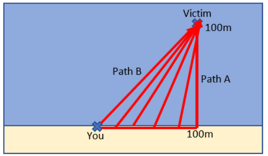
You might think that we are done, since we figured out that Path A is better than B, but we have just scratched the surface of the lifeguard problem. Figure 2.2 shows that there are not only two paths. You can dive in immediately or run 100 meters and then swim or choose any distance in between! The problem is to find the best, fastest path.
The lifeguard problem can be solved analytically, with calculus and algebra, but we will not do that. Instead, we will use numerical methods: An algorithm is used to get an approximate result. We will implement the problem in Excel and use Excel’s Solver add-in to find the correct answer.
STEP Open a blank Excel workbook and save it as LifeguardProblem.xlsx. Enter the numbers and labels shown in Figure 2.3. Make sure your Excel workbook looks exactly like Figure 2.3 because we will be referencing those specific cell addresses.
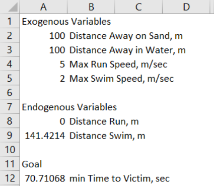
Exogenous variables cannot be changed by the decision-maker. From the Greek, exo means “outside,” like a lobster’s exoskeleton. Exogenous variables are outside or beyond our control. They are also known as independent, given, or constant variables. They are parameters that are part of the decision-maker’s environment.
You certainly cannot control where the victim is drowning. If you could, the problem would be trivial—you would put them right at your feet and pull them out. So the location of the drowning swimmer is exogenous: 100 meters away on the sand and 100 meters from the shore in the water.
Your run and swim speeds are also exogenous. You might think you can control how fast you run and swim, but these are not the actual variables. As the labels show, “Max Run Speed” and “Max Swim Speed” are your fastest run and swim speeds. We are assuming you are going all out to save the victim. Sure, you could train to get faster, but at that moment when you are trying to save the victim, your max speeds are given. The fastest you can (and will) run is 5 m/sec, and the fastest you can (and will) swim is 2 m/sec.
To really cement the concept of exogenous variables, ponder this: If you were waiting to order at the drive-thru at your favorite fast-food restaurant, could you think of a few exogenous variables? What makes the variables you chose exogenous?
Endogenous variables are the ones the decision-maker sets and determines. Since endo means “inside” in Greek (you have an endoskeleton), endogenous variables are within your control. They are also known as choice or dependent variables. What to drink is endogenous to you at the fast-food restaurant.
You decide how far you will run from zero (dive right in and start swimming, Path B) to 100 meters (Path A), so this is the endogenous variable in this problem. Notice that deciding how far to run immediately determines how much you will swim, since you will always swim in a straight line along the hypotenuse formed by the triangle of where you entered the water (see Figure 2.2). We can use Excel to demonstrate this.
STEP Enter the formula =SQRT((A2-A8)ˆ2+A3ˆ2) in cell A9 and press Enter. You will know you did it correctly if Excel displays something close to 141.4217. The formula computes the hypotenuse for any value of cell A8. Excel treats the value of the blank cell A8 as zero, so A2 − A8 is 100 and we get the hypotenuse of Path B (shortest total distance).
EXCEL TIP Maximize the flexibility of your spreadsheets.
It would have been easier to enter and read the formula if we hard-coded the distance away on sand and in water like this: =SQRT((100-A8)ˆ2+100ˆ2), but we would lose the flexibility of being able to change these variables and have the formula automatically update. In general, you want to develop spreadsheets that depend on other cells and not on numbers.
STEP To make sure the formula works well, let’s check Path A: Enter 100 in cell A8. Cell A9 should also display 100. If not, return to the previous step and fix the formula.
In addition to exogenous and endogenous variables, every optimization problem has to have a goal, known more formally as an objective function. For the lifeguard problem, this is minimizing the time it takes to get to the victim. The goal always has to be a function (in Excel, a formula) that depends on the endogenous variables.
STEP Enter the formula =A8/A4+A9/A5 in cell A12 and press Enter. You will know you did it correctly if Excel displays 70 (with cell A8 at 100), since we know this is how long it takes for Path A.
Having set up the optimization problem in Excel with exogenous and endogenous variables, along with a goal, we are now ready to find the best path. We begin by manually trying a few different paths.
STEP Set cell A8 to 50 and notice the time to victim. Try 25 and 75. Keep playing with cell A8 until you think you’ve found the best answer.
Cell A8 should now be in the mid-50s, and the time to victim should be around 65.8 seconds. That’s several seconds better than Path A or B—this could mean the difference between life and death!
Not many people try fractional distances, but this is perfectly acceptable. Of course, we are not going to hunt and peck for hours, changing A8 by 0.001 to see the effect on A12. Instead, we will use Excel’s Solver. Hunting and pecking (or its twin, plugging and chugging), but really fast, is exactly what Solver does.
Excel’s Solver is an optimization algorithm. It tests many trial solutions very quickly, converging to an answer. Later, we will explore how it works in more detail. Right now, let’s see it in action.
STEP Click the Data tab (in the Ribbon across the top of the screen), then Solver (in the Analysis group) to bring up the Solver Parameters dialog box. If Solver is not available, then use the Add-in Manager to install it. Use Excel’s Help if you are having trouble or visit support.office.com.
EXCEL TIP Press Alt, t, i to access the Add-in Manager. Press the Alt key, then release it and press the letter t, then release it and press the letter i to quickly bring up the Add-in Manager.
The Solver Parameters dialog box is initially empty. You need to give it the appropriate information before asking it to search for a solution. It always needs specific cell addresses for the Objective and Changing Variable Cells inputs. Some problems are constrained and require further input, but the lifeguard problem does not.
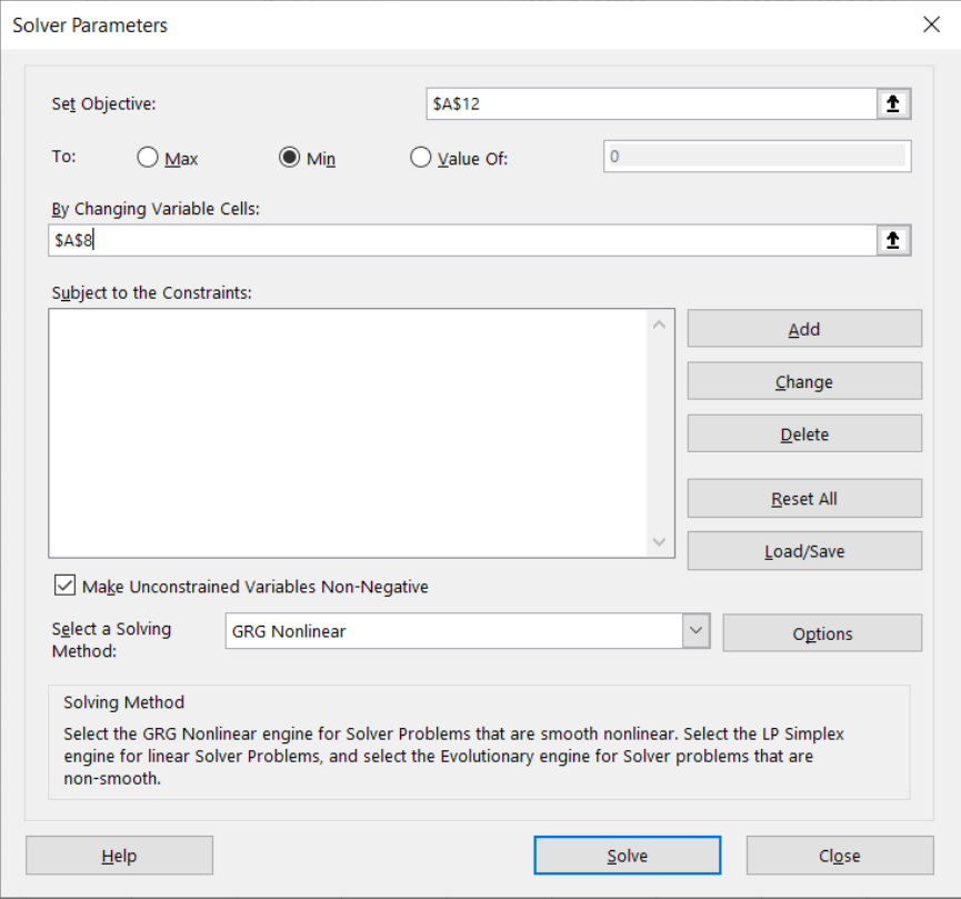
STEP Do these three things: (1) Click in the Set Objective input field and select cell A12 by clicking on it. (2) Click the Min radio button. (3) Click the By Changing Variable Cells input field and select cell A8. Your screen should look like Figure 2.4. If not, make it so.
Source: Screenshot of Excel interface, © Microsoft Corporation.
STEP Click the Solve button in the bottom-right corner of the Solver dialog box, read the Solver Results dialog box, and click OK.
You did it! You found the correct answer to the lifeguard problem! By running about 56 meters before jumping in, you will reach the victim in a little under 66 seconds, and this is the shortest possible time. We can see that this is a true minimizing solution by exploring a small move away from Solver’s solution.
STEP Change cell A8 to 57 and you can see that cell A12 increases a little bit. Decrease cell A8 to 55 and, once again, cell A12 goes up. That is pretty convincing evidence that Solver has the correct answer, since the values around it yield higher times to reach the drowning person.
There is more to do, but let’s recap. We modeled an optimization problem, implemented it in Excel, and used Excel’s Solver to find the optimal solution. There are other ways to solve optimization problems, but Solver offers a pretty simple approach—as long as you can set up the problem in Excel, Solver has a shot at solving it. We will see in future work that Solver is not perfect, but on a simple problem like this one, it is reliable.
Excel’s Solver is an example of numerical methods. Its answer is not exactly correct, but it is so close that, practically speaking, it is the right answer. This problem can be solved analytically to get an exact solution, and doing so yields something called Snell’s Law. Physicists have known for a long time that light refracts when it goes through a different medium than air, like water. As Pierre de Fermat realized in 1650, light is taking the fastest path, and this is why it bends when it hits water.
There are some pretty mind-boggling applications of minimizing time across different media from the natural world. Some people think dogs can find the optimal path (Pennings, 2003; Perruchet and Gallego, 2006) and so can ants, as shown in Figure 2.5. As described in the caption, the green area is rough felt that is harder to walk on. The ants do not go in a straight line to the food (like they do in a control setting with only the white, smooth surface). The authors call this decentralized optimization because the ants are working together without any direction from an authority telling them what to do.
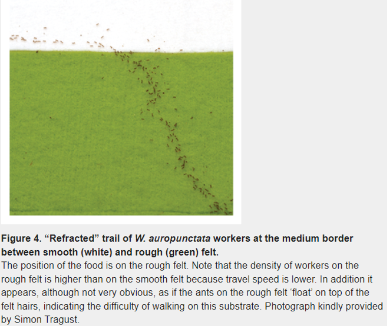
Source: Oettler et al., 2013 / CC-BY.
Let’s close with a crazy thought experiment. What would happen if you were suddenly transformed from a slow runner and near-Olympic swimmer to a freakish mix of Usain Bolt and Michael Phelps? Not only are you a really fast swimmer, but you also can run 100 meters in 10 seconds, so your maximum run speed is a blazing 10 m/sec. How does this shock (change in the maximum run speed exogenous variable) affect your decision of how far to run?
STEP Change cell A4 to 10 and run Solver.
Does Solver’s new optimal solution make sense when compared to the initial answer?
Takeaways
We introduced and solved the lifeguard problem: To get to a drowning swimmer as quickly as possible, the lifeguard has to choose the best path.
This is a well-known problem in physics and optics because light bends (refracts) when it goes through a different medium, like when it hits water.
There are several different analytical formulas, but we used Solver (a numerical method) to find the fastest path.
We had to implement the problem in Excel, creating an objective function that depended on a changing (endogenous variable) cell and constant (exogenous variable) cells. We then called Solver, and it generated the correct solution.
References
The epigraph of this chapter can be found in section 26-3 of the online edition of Feynman’s famous Lectures on Physics. He explains what Fermat did and gives the analytical solution. The lectures are freely available from Caltech’s website (where he taught for many years): https://www.feynmanlectures.caltech.edu/.
For a fun visualization of the lifeguard problem, see geogebra.org/m/wBcKASpN.
Oettler, J., Schmid, V., Zankl, N., Rey, O., Dress, A., and Heinze, J. (2013). “Fermat’s Principle of Least Time Predicts Refraction of Ant Trails at Substrate Borders.” PLOS One, open access: doi.org/10.1371/journal.pone.0059739.
Pennings, T. (2003). “Do Dogs Know Calculus?” College Mathematics Journal 34, no. 3 (May 2003), pp. 178–182, jstor.org/stable/3595798.
Perruchet, P., and Gallego, J. (2006). “Do Dogs Know Related Rates Rather Than Optimization?” College Mathematics Journal 37, no. 1 (Jan. 2006), pp. 16–19, www.jstor.org/stable/27646266.
2.2 Visualizing Comparative Statics
When maximum run speed increases from 5 to 10 m/sec, you run longer and dive in after running nearly 80 meters. Thus, you run roughly 23 meters more than when your max speed was 5 m/sec. This is about a 40% increase (=23/56). Running more (and swimming less) makes sense—after all, you are much faster running now that you are a world-class sprinter, so you should take advantage of this.
Changing an exogenous variable while holding everything else constant (called ceteris paribus) is known as comparative statics analysis. It is comparative because you are comparing the new to the initial optimal solution, and it is statics because you focus only on the beginning and the end, ignoring any kind of adjustment process (which, if not ignored, would be dynamic analysis).
One way to understand what we are doing is by creating a simple graph to show the optimal solution. The x-axis will be how far we run before diving in, and the y-axis will be the corresponding time.
STEP Using the initial problem (make sure cell A4 is set to 5), enter the labels Distance Run, Distance Swim, and Time to Victim in cells G1, H1, and I1, respectively. Create a series from 0 to 100 by 5 by entering 0 in cell G2, 5 in cell G3, and then filling it down by selecting cells G2 and G3, clicking on the bottom righthand corner of cell G3, and dragging down. In cell H2, enter the formula for the hypotenuse based on the value in cell G2. Fill down. Compute the Time to Victim in cell I2 and fill it down. Check your numbers with Figure 2.6, and if there are any discrepancies, fix your formulas or, if you cannot do it, proceed to the appendix to get help.
Now that we have data for how Time to Victim responds to Distance Run, we can visualize the lifeguard problem by creating a chart. You may know how to make a chart in Excel, but it is worth reviewing basic charting principles before diving in.
STEP Watch this three-minute video on making a chart in Excel: vimeo.com/econexcel/how-to-chart-in-excel.
Selecting data, clicking the desired chart type, and cleaning up the chart are the three steps. Always check the axes and titles and avoid the dreaded “Series 1” legend text like the plague. Stay away from chart junk (wild colors and crazy fonts). Best practice is minimalist—let the data speak for itself (Tufte, 1983).
STEP Make a Scatter chart of Time to Victim as a function of Distance Run. Check that your chart looks like Figure 2.6.
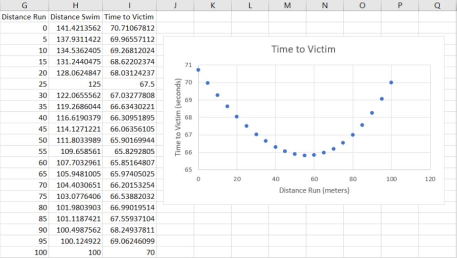
Figure 2.6 shows pretty clearly that the optimal solution is at the bottom of the U-shaped Time to Victim function. The lifeguard really does face an optimization problem. Correctly solving it means the lifeguard will get to the drowning person as fast as possible.
We can highlight the optimal solution and learn how to add controls to a spreadsheet. The Developer tab needs to be visible on the Ribbon. If it is not, click File, then click Options, then click Customize Ribbon, and check the Developer item.
With the Developer tab available in the Ribbon, we are ready to add a scroll bar. First, we will get a coordinate point, then we will add it to the chart, and finally, we will connect it to a Scroll Bar control.
STEP Select cell range G22:I22 and copy (Ctrl-c), select cell G24, and paste (Ctrl-v). In cell G24, enter the formula =A8 so that we have the optimal solution.
To add this single point to the chart, we will use a powerful, advanced method: We will directly edit the SERIES formula. This approach allows you to easily and quickly reuse or update a chart.
STEP Watch this five-minute video on how to modify the SERIES formula in a chart: vimeo.com/econexcel/using-series-formula.
We can now add the single point to the chart by copying the existing SERIES formula and editing it, replacing the x– and y-axes data with the cell addresses of the single point.
STEP Click on the Time to Victim series (click on one of the points), copy, press the Esc key (to clear the formula bar), click on the northwest corner of the chart, paste, and then edit the SERIES formula so it looks like this:
=SERIES(Sheet1!$I$1,Sheet1!$G$24:$G$24,Sheet1!$I$24:$I$24,2)
Notice the 2 at the end—this ensures that the point is always visible because it is on top of the first series. To highlight it further, increase the size of the point by clicking on it and increasing the width of the marker size to 5 pts.
You can enter any number from 0 to 100 in cell A8 to display that point on the Time to Victim function. We can make it easy for the user to move the point on the chart by adding a scroll bar connected to cell A8.
STEP Click the Developer tab on the Ribbon, click the down arrow in the Insert button, and select the scroll bar icon (in the top, Form Control group) as shown in Figure 2.7. Click and drag on the spreadsheet (roughly under the chart) to create the Scroll Bar control.
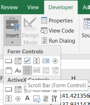
Source: Screenshot of Excel interface, © Microsoft Corporation.
STEP Right-click the Scroll Bar control (that you just created), click the Control tab, click in the Cell link field, and click cell G24 (it appears in the field). Click OK and click on a cell in the spreadsheet. Click a few times on the scroll bar to make the red dot on the chart move along the Time to Victim function.
You can also click the scroll box itself (sometimes called a thumb) and drag it. You can also manually change the value in cell G24, and the scroll bar box will reflect that value.
STEP Enter the formula =A8 in cell G24 to display the optimal solution and see that the scroll box moves to this value.
We now have a clear display of the optimal solution and understand that it minimizes Time to Victim, but the correct solution depends on the exogenous variables. What happens, for example, when you become Usain Bolt and can run not 5 m/sec but 10 m/sec?
STEP Change cell A4 to 10 and watch what happens.
Excel immediately updates the chart, and the changes are dramatic. It is clear that the function has shifted down, and there is a new minimum to the right of the initial solution.
How can we compare the two situations? One way is by displaying the two environments (initial with 5 m/sec and new with 10 m/sec) on the same chart. We can do this with a clever trick that has many applications: Create a transparent image and lay it on top of the chart.
To make the comparison display correctly, we need to lock down the y-axis in the chart.
STEP Right-click any number on the y-axis, and change the minimum and maximum axis bounds to 55 and 75, respectively. Change the major unit to 5.0.
If the aforementioned step is skipped, the “chart stacking” strategy will not work because Excel will automatically adjust the y-axis scale. Manually setting and fixing the scale is a necessary step when stacking charts.
STEP Click the chart, click the Format tab in the Ribbon, click Shape Fill, and select No Fill. Click and drag the chart around a little to see that it is transparent.
The cell borders are now visible, and this is distracting, so we will remove them.
STEP Click Page Layout in the Ribbon and uncheck View under Gridlines (in the Sheet Options group).
The chart is still transparent, but there are no cell borders, so the chart’s background is white.
STEP Select and copy the chart, then click on a cell (to unselect the chart). Click the down arrow on the Paste menu item (in the Home tab) and click on the picture icon as shown in Figure 2.8.
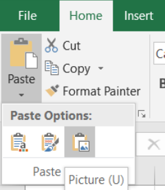
Source: Screenshot of Excel interface, © Microsoft Corporation.
The chart you just pasted is “dead” in the sense that it is a fixed image and is not connected to the data like the original chart. It can be pasted into a doc or slide and will not change even if you alter the data.
STEP Drag the chart you just pasted so it is exactly on top of the live, original chart. Add text boxes to label the initial and new solutions (remove the border and fill of the text boxes to improve the display).
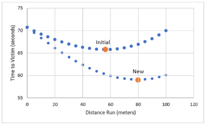
Your final product should look like Figure 2.9. It clearly shows the impact of the shock to running speed on the lifeguard problem. The entire function shifts down, and the minimum moves to the right.
What other exogenous variables are there in the lifeguard problem that we ignored? Imagine yourself as a real lifeguard on a crowded beach, perched on a chair, looking out over the ocean. What else would influence your decision of where to enter the water?
Takeaways
We shocked the lifeguard problem by changing max run speed from 5 m/sec to 10 m/sec, ceteris paribus, and found that the optimal distance to run on the sand increased. This is an example of comparative statics analysis.
We visualized the lifeguard problem by creating a chart in Excel of Time to Victim as a function of Distance Run. This made it easy to see that we are working on a minimization problem and that the solution is at the bottom of the bowl.
Creating a chart in Excel always involves three steps:
-
- Select the data: Hold down the Ctrl key to select noncontiguous cells.
- Insert the desired chart type: Usually it is a Scatter chart, but Excel has many chart types.
- Clean up the chart: Be sure to check the title, the legend text, and the axes labels.
Data visualization is a mixture of art and science. In Excel, always remember the third step in charting: label axes, add a descriptive title, and make sure the chart is clear and easy to understand. Be sure that the legend is needed and makes sense. A minimalist approach is best.
The bible of chart design is Tufte (1983). This classic preaches simple, clean chart design. Excel allows you to do all kinds of word art and color schemes. You should avoid this.
Excel is complicated software with many features and capabilities. Understanding that a chart is really a SERIES formula is a big step forward. Directly editing the SERIES formula has many powerful applications.
The transparency trick is also quite useful. You are slowly building a library of skills and knowledge. There is not a single, specific thing that makes you an Excel expert. It is like a wall; every brick matters.
References
Barreto, H. (2013, July 2). How to Chart in Excel [Video]. Vimeo. vimeo.com/econexcel/how-to-chart-in-excel.
Barreto, H. (2012, March 9). Using SERIES Formula [Video]. Vimeo. vimeo.com/econexcel/using-series-formula.
Tufte, E. (1983). The Visual Display of Quantitative Information (Cheshire, CT: Graphics Press), open access: archive.org/details/visualdisplayofq0000tuft.
For more on how graphs and data visualization evolved, see Friendly, M., and Wainer, H. (2021). A History of Data Visualization and Graphic Communication (Cambridge, MA: Harvard University Press).
Appendix
To replicate Figure 2.6, follow the steps here, but think about the formulas you are entering and what each cell is doing instead of mindlessly typing:
(1) In cell H2, enter the formula =SQRT(($A$2-G2)ˆ2+$A$3ˆ2) and fill it down. Note that if you do not use absolute references (the $ before cell column and row), then the formula does not work when you fill it down.
An absolute reference, like $A$2, means when you copy and paste the cell (or fill it down), the formula remains unchanged and will continue to refer to $A$2. A relative reference, like G2 (no $ signs), means the formula will change because entering =G2 in cell H2 means “the cell one column to the left of this cell.”
(2) In cell I2, enter the formula =G2/$A$4+H2/$A$5 and fill it down. Again, note the use of absolute references.
Both formulas were used earlier and neither hard-code the variables—in other words, cell addresses are used instead of numbers. This maximizes spreadsheet flexibility.
Use the Ctrl key to select noncontiguous data to make the chart.
2.3 Solver Pros and Cons
We know Solver is a numerical methods (as opposed to analytical) approach to solving an optimization problem. We saw it in action as it minimized the time it takes to reach the victim in the lifeguard problem for running speeds of 5 m/sec and 10 m/sec.
This section is devoted to these two questions:
-
-
- How does Solver actually work?
- Can we always count on it giving us the correct answer?
-
The answer to the first question is explored in more detail in the next section, but in a nutshell, Solver hunts and pecks really fast and converges to a solution. The answer to the second question is shorter: no. We will see that Solver can fail in two ways: miserable and disastrous. It can announce that it cannot find the answer (that is miserable), or worse, it can claim to have an answer that is wrong. This is disastrous because you think it is right, but it is not. The bottom line is that you always need to be on high alert when using Solver—it is not a silver bullet.
How Does Solver Actually Work?
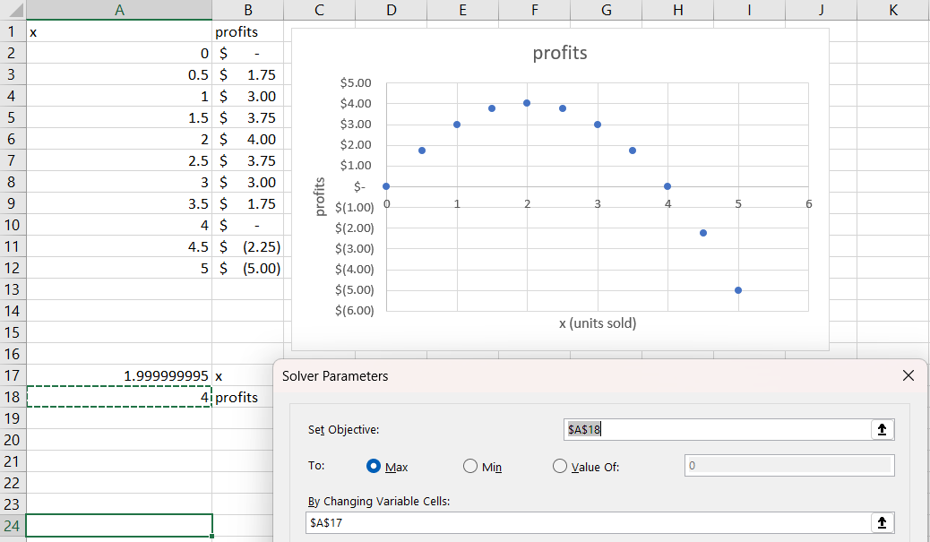
We begin our explanation of how Solver works with a simple profit maximization problem. A firm sells its product at $4/unit, and it has costs of production given by the square of the number of units it produces. So it costs $9 to make 3 units and $25 to make 5 units. Since the price is $4, the firm’s revenue function is 4x. If it sells 3 units, it makes $12, while 5 units generate $20 of revenue.
The firm seeks to maximize profits (denoted by convention with the Greek letter pi, π), which are equal to revenues minus costs. The following profit function says that 3 units produce $3 of profit ($12 of revenue minus $9 of costs), and 5 units leave the firm with a loss of $5, since 20 − 25 = −5.
[latex]\underset{x}{max \pi} = 4 x - x^{2}[/latex]
If you know calculus, you could solve this problem analytically by taking the derivative with respect to x, setting it equal to zero, and solving for x*. But even without calculus, the solution is obvious if you tabulate (a single-entry table that lists the values of a function at discrete points) and graph the profit function.
STEP Create data and make a chart of the profit function with the x-axis going from 0 to 5 in increments of 0.5. If you have trouble, see the appendix.
Both the data you created and the corresponding chart show that the answer is x* = 2, leading to maximum profits of $4. Can Solver also find the optimal solution? Yes, it can.
STEP Use cell A17 for x, and enter the profit formula in cell A18. Next, call Solver and fill in the dialog box and click Solve. Again, if you have trouble, see the appendix.
As expected, Solver finds the optimal solution, but how does Solver do it? In a word, iteration, which means repetition. Solver runs the following three steps over and over until it cannot improve much:
-
- Using the starting value in cell A17 (this is zero if left blank), it evaluates cell A18.
- It then moves away from the starting value. The amount it moves is determined by the particular recipe—a popular one (and Solver’s default) is called Newton-Raphson steepest descent.
- It compares the new value of profits to the original. If profits are higher, it continues in that direction. If lower, it goes in the opposite direction.
Solver continues iterating, changing cell A17 and checking how profits respond, until the improvement in profits is “small,” an amount determined by the convergence criterion. The last change it made to cell A17 is the answer.
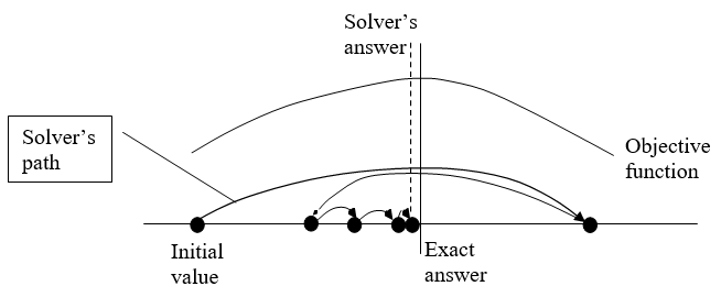
The stylized graph (which means it represents an idea without using actual data) in Figure 2.10 shows that Solver works by trying different values and seeing how much improvement occurs. The path of the choice variable (on the x-axis) is determined by Solver’s internal optimization algorithm. See FrontlineSolvers at https://www.solver.com/excel-solver-online-help to learn more about Excel’s Solver.
When Solver takes a step that improves the value of the objective function by very little, determined by the convergence criterion (adjustable via the Options button), it stops searching and announces success. In Figure 2.10, Solver is missing the optimal solution by a little bit because, if we zoomed in on the graph, the objective function would be almost flat at the top. When Solver computes minuscule additional improvement, it stops and announces it has found a solution.
This is all too abstract. Let’s see it in action.
STEP Set cell A17 to 1.1 and widen column A to make sure it displays many decimal points. Call Solver, but this time, click the Options button and check Show Iteration Results (in the All Methods tab). Click Solve. Click Continue as many times as needed and watch the values on the spreadsheet.
Excel displays each trial solution. Solver might (this is not guaranteed) even hit 2 as a trial solution, but then it moves off it because it does not know this is the exactly correct answer.
It is quite likely that, starting from 1.1, Solver’s answer is not exactly 2. You might have a result like this: 1.99999999467892. When we say Solver got the answer, we mean this in a practical sense. If Solver is off from the exact answer by a tiny amount, that is success, for all practical purposes.
There is a danger to avoid when using Solver (or any numerical optimization method that relies on convergence): It is easy to conclude that Solver must give an exact answer because it displays so many decimal places. This is incorrect. Solver’s solution is an example of false precision. It is not true that the many digits provide useful information. The exact answer is 2.
Usually, Solver does not find the exactly correct answer, yet it displays a number with many digits. This is Solver noise (a less technical way of saying “false precision”). You must learn to interpret Solver’s results as inexact and not report all the decimal places. You must use words like roughly or approximately when reporting answers produced by Solver.
In general, there are two reasons for really tiny disagreements between Solver and the exact answer.
1. Excel cannot display a number to an infinite number of decimal places. Most modern Excel software has 15 significant digits of precision. If the solution is a repeating decimal or irrational number, there is no exact decimal representation. Even if the number can be expressed as a decimal—for example, one-half is 0.5—precision error may occur during the computation of the final answer.
STEP Click in any cell and enter the formula =pi(). Now select the cell displaying π and add decimal places by repeatedly clicking the Increase Decimal button ![]() , in the Home tab of the Number group in the Ribbon. When Excel displays “######,” it means the number does not fit in the column, so you need to widen the column. Keep adding decimal places until you start seeing zeroes. You have reached Excel’s maximum precision.
, in the Home tab of the Number group in the Ribbon. When Excel displays “######,” it means the number does not fit in the column, so you need to widen the column. Keep adding decimal places until you start seeing zeroes. You have reached Excel’s maximum precision.
2. Even if the answer is an integer, like 2, Excel’s Solver often misses the exactly correct answer by small amounts. Solver’s convergence criterion (that you can set via the Options button in the Solver Parameters dialog box) determines when it stops hunting for a better answer. Excel treats all numbers the same—it has no way of saying, “Oh, that’s really close to 2, so the answer must be 2.”
False precision or Solver noise is a serious issue. Be aware that Solver’s answer is likely not the exactly right answer. There are other ways in which Solver can fail us that are more serious than misunderstanding precision.
Solver Behaving Badly
A miserable result (an actual technical term in the numerical methods literature) occurs when an algorithm reports that it cannot find the answer or displays an obviously erroneous solution. We can easily create an example.
STEP Copy your existing sheet (right-click the sheet tab in the bottom left-hand corner, select Move or Copy . . . and check Create a copy). Select cell B2 and delete the -A2ˆ2 part of the formula so you have only =4*A2. Fill down.
The chart updates and you have a straight line. You are graphing total revenue now instead of profits.
STEP Select cell A18 and change the formula to =4*A17 (just like you did to the chart). Call Solver and click Solve.
You are looking at a miserable result. Solver cannot find a solution, so it announces (loudly, with a red exclamation mark) that it cannot find an answer.
In this case, that is actually reasonable. After all, this function does not have a well-defined maximum, unless you want to argue that the answer is positive infinity.
Solver will also give a message like this if it cannot perform a computation such as dividing by zero or taking the square root of a negative number. The algorithm fails, which is bad news, but at least it tells you that it cannot solve the problem.
When Solver fails like this, there are three basic strategies to get Solver to find a solution (but nothing is guaranteed):
- Try different initial values in the changing cells. If you know roughly where the solution lies, start near it. Always avoid starting from zero or a blank cell.
- Add more structure to the problem. Include nonnegativity constraints on the endogenous variables, if appropriate.
- Completely reorganize the problem. Instead of directly optimizing, you can put Solver to work on conditions that must be met.
None of these approaches will work on this problem because it does not have a solution.
There is a second way in which Solver can behave badly, and it is much worse than a miserable result. Solver can give an answer that is wrong, yet it thinks it is right and reports it as the solution. This is called a disastrous result. Again, we can create an example to demonstrate this.
Our example requires use of a more complicated cost function. Instead of the simple square we used earlier, we will use a cubic cost function, ax3+bx2+cx. By strategically choosing the coefficients a = 1, b= −8, and c = 19, we can get a cost curve that will give us a profit function with a trough and a peak, like a sine wave:
[latex]\underset{x}{max} \pi = 4 x - ( \left(x^{3} - 8 x^{2} + 19 x\right) ) = 4 x - x^{3} + 8 x^{2} - 19 x[/latex]
STEP Copy the original sheet again. Change cell B2’s formula so it looks like this: =4*A2-A2ˆ3+8*A2ˆ2-19*A2. Fill it down.
The graph updates and now has a clear maximum near x = 4 but also has a valley as we increase output starting from zero. Can Solver find the optimal solution with this more complicated cost function?
STEP Edit cell A18 so that it uses the new profit function. The formula should look like this: =4*A17-A17ˆ3+8*A17ˆ2-19*A17. Call Solver and click Solve. How did it do?
If you started from the original sheet’s optimal solution (x = 2) or near the maximum, then Solver will work fine. Notice that Solver’s answer is a little higher than 4, and remember that Solver’s answer is not the exact optimal solution, but it is really close (off by 0.000001 or so).
STEP Change cell A17 to 1 and run Solver. What happens now?
You just saw a disastrous result. Solver said it got an answer, but it is wrong. Your spreadsheet is showing that cell A17 is zero, but we know the correct solution is a little over 4. This is really bad and shows that we must always be skeptical of Solver. It is not a silver bullet, and mindless reliance on its output is a recipe for disaster.
Can you figure out why Solver failed?
STEP To help you, look at the chart and remember that we started from x = 1. Force your eyes to follow a straight line down from 1 (on the horizontal axis). You can see that you are to the left of the minimum of the profit function.
The fact that we are on a downward-sloping part of the profit function explains why Solver failed. It started from there, and the algorithm led it away from the true max (x becoming smaller) because profits rise (become less negative) as x decreases.
We can see that starting from near the maximum generates a good result because the function is a hill around the maximum. Moving away leads you to lower profits so the algorithm can find the correct solution.
STEP Start from 7 (set cell A17 to 7) and run Solver to see that starting values around the top of the hill enable Solver to succeed.
Will any starting value far away from zero work?
STEP Start from 100, then try 10.
This is surprising. If you start too far from the maximum, Solver takes a big first step that leads it to the wrong answer. Notice, however, that Solver does not give any indication that something may be wrong. To be clear, with a disastrous result, the computer’s answer is incorrect, but you have no way of knowing this. That means you always have to be skeptical and vigilant when using Solver.
Unlike a miserable result, where we know we have a problem, a disastrous result tricks us into thinking all is well. Even when Solver says it has an answer, you should question it. Try starting from a different place to see if you get the same answer. Always ask yourself if the answer makes sense. Be careful out there.
Takeaways
Solver is an example of a search algorithm. It works by exploring the objective function, like an ant crawling on a surface. If movement in a certain direction improves things, then it keeps going that way. Moves that generate worse results lead to it reversing course.
Usually, this is an effective method. Many problems have solutions that can be found by numerical methods, using a computer to plug and chug through the problem.
Even when Solver finds the solution, always remember that its answer is not likely to be exactly correct. Solver usually suffers from what is formally known as false precision (and we call it, intuitively, Solver noise). This means that the last decimal places are not reliable and do not signal exactitude.
You want to be a sophisticated user and understand that, while powerful, Solver is not perfect. It can fail in two ways:
- A miserable result is when Solver surrenders and announces that it cannot find an answer. This is disappointing.
- A disastrous result is much worse. Solver says it has an answer, but it is wrong. This happens when you have a difficult problem, perhaps like asking an ant to find the highest point on a crumpled piece of paper. It is likely to find a local maximum but not a true, global max.
Solver is a tool, like a chain saw. You can use it to cut down and trim trees really fast. You can also cut your leg off with it. Be careful.
Appendix
Charting the Profit Function
To make a chart of the profit function, begin with x-axis data. Create a label in cell A1 by entering the letter x. Below it, enter a 0, then a 0.5 below that. Select both cells, then fill down to cell A12, which should display 5.
For the y-axis, enter the label, profits, in cell B1. In the cell below it, enter the formula =4*A2-A2ˆ2. Fill it down. Format the profit values as $.
Select the data and make a Scatter chart. Remember to add labels for the axes and an appropriate title. Your chart should look like Figure 2.11.
Using Solver to Find the Optimal Solution
Enter the labels in cells B17 and B18 shown in Figure 2.11. Enter the formula =4*A17-A17ˆ2 in cell A18. Call Solver (click the Data tab in the Ribbon and click Solver), then click on cell A18 for the objective function and cell A17 for the changing cells (as shown in Figure 2.11). Click Solve and click OK when Solver displays its Results dialog box.
Source: Screenshot of Excel interface, © Microsoft Corporation.
2.4 Profit Maximization Practice Problem

Source: Stable Diffusion, 2023/ License.
You are a farmer. You buy seed, do a lot of work (till the soil, plant, irrigate, fertilize, and control weeds), then harvest and sell your crop. To keep the optimization problem simple, we assume away almost all of this and ignore all labor, all machinery, and any other costs except seed.
In our toy model, you simply buy seed, S, and it is transformed into output—say, corn—via the function [latex]Q=100\sqrt{S}[/latex]. For example, 64 pounds of seed makes 800 pounds of corn, 100 times the square root of 64. This functional form reflects the fact that you have a fixed amount of land, so planting twice as much seed less than doubles the amount of corn. The square root means that more seed increases output, but at a decreasing rate.
You sell your output at the market-given price, P, of $8 per pound. You cannot sell at a price higher than this because there are many other farmers willing to sell at $8 per pound, so no one would buy your harvest at a price above the market price. To be clear, 1,000 pounds of corn generates $8,000 of total revenue.
The seed costs you $2 per pound. You can buy as much seed as you want at this price, so your total cost function is linear, TC = $cS, where c is the input price of seed. The total cost function tells us that, for example, 200 pounds of seed has a total cost of $400.
You want to buy the amount of seed that maximizes profits, which is total revenues minus total costs. You can see that choosing 100 pounds of seed will get you $8,000 − $200 = $7,800 of profits.
The question, however, is whether or not that’s the best amount of seed to buy—in other words, is 100 pounds of seed the profit-maximizing solution? The following questions will lead you to an answer to this question and help reinforce what you know about Solver, data visualization, and comparative statics analysis.
STEP Open a blank Excel workbook and save it with an appropriate file name. Answer the following questions in the spreadsheet, saving the file after each question (in case there is a crash or other problem). For questions that require explanation, put your response in a text box (in the Insert tab on the Ribbon) with the question number.
- What is the endogenous variable in this problem? Why is it endogenous?
- Put the values for the output price of corn and the input price of seed in two cells with labels next to them.
- Implement this problem in Excel so that it is ready for Solver to work on it. You do this by adding other information in cells in addition to the cells you have from the previous question.
- Use Solver to get the optimal solution.
- The exactly correct answer is 40,000 pounds of seed with maximum profits of $80,000. Since Solver does not give this exactly correct answer, do we say it is wrong? Explain.
- Create a chart that displays the optimal solution.
- What are the three steps in creating a chart in Excel? Did you do all three steps in the chart you made?
- We know Solver can give miserable or disastrous results. What do these terms mean?
- Does your chart give you confidence that Solver is not giving a disastrous result in this case? Explain.
- Conduct a comparative statics analysis of changing the output price. Explain what you did and what you found.
RAND()
For the last question, you can change the output price to any number you choose, but you could also use Excel to generate a random number for the output price using the RAND() function. We will explain and use RAND() in chapter 3, but it is very easy to use and gives you a way to play with the exogenous variables in this problem, so it is worth doing it now.
STEP In any empty cell, enter the formula =RAND() and press Enter. Press the F9 key (you may have to use the function, fn, key to access F9 on your keyboard) repeatedly to see the number bounce around.
EXCEL TIP The F9 key is a keyboard shortcut for Calculate Now in the Formulas tab in the Ribbon. It recalculates the sheet and updates functions like RAND(), thereby displaying a new random number.
You cannot run Solver with an objective function that depends on RAND() because every time Solver puts down a trial solution, the cell with RAND() would recalculate. There are, however, several ways to “deaden” RAND() and turn it into a number. Perhaps the easiest uses the F9 key when you are in the formula bar of the cell.
STEP Copy your RAND() cell and paste it into another empty cell. Press F9 repeatedly to see two bouncing numbers. Select one of the cells with RAND() and then click in the formula bar. Press F9 and then Enter.
You replaced the formula in that cell with a single number that will no longer change when the sheet recalculates. You could create a cell formula for the output price like =RAND()*4+6 to generate random output prices from 6 to 10. You could get a specific, unchanging price by entering the formula bar of that cell and pressing F9. You can make many practice problems with different output prices with this method.
