
8 National Income Accounting
The NIPAs trace their origin back to the 1930s, when the lack of comprehensive economic data hampered efforts to develop policies to combat the Great Depression. In response to this need, the U.S. Department of Commerce commissioned future Nobel Laureate Simon Kuznets to develop estimates of national income.
Bureau of Economic Analysis (BEA) documentation
8.1 GDP and Macroeconomic Volatility
Just like a business needs an accounting system to keep track of what is going on, the National Income and Product Accounts (NIPAs) measure how the economy is doing. Before the 1930s, policy makers were flying blind—no one really knew how the economy was performing.
Gross domestic product (GDP) is the market value of all final goods and services produced within a country in a given period of time. This is the most fundamental measure of economic activity.
The bedrock accounting equation is GDP = C + I + G + NX. There are several ways to compute GDP, but this equation focuses on spending. It says that GDP can be computed as the sum of consumption (C), investment (I), government (G) spending, and net exports (NX).
STEP Open Excel and save a workbook as GDPInvestment.xlsx. Enter these Series IDs in the top row: GDP, PCEC, GPDI, GCE, and NETEXP. Use the FRED Excel add-in to get the data (refer to previous work with FRED if needed). In cell K8, enter the formula =B8-D8-F8-H8-J8. That is GDP − C − I − G − NX. Display three decimal places.
Excel shows 0.000—GDP really and truly is the sum of spending by consumers, firms, and governments (local, state, and federal) plus net exports.
STEP Fill cell K8 down. Scroll down and look at the values.
Yes, GDP = C + I + G + NX is always true, with a little rounding error—a small numerical discrepancy. For example, adding 1.3 and 1.6 gives 2.9. If we round to the integer before adding, we get 1 plus 2 equals 3. Rounding errors are often found when the sums of percentages are slightly more or less than 100% in a table.
With three decimal places displayed, you can see that sometimes column K shows a plus or minus 0.001. That is a rounding error in the GDP aggregates (C, I, G, and NX).
GDP is a flow, not a stock. GDP measures output per time period (usually a quarter or a year), not a total accumulated at a point in time. Imagine water flowing into a bathtub—GDP is how much water is pouring in (so liters or gallons per minute), not how much water is in the tub.
C, I, and G are the total spending (purchased final goods and services) made by consumers, firms, and governments, respectively. A computer can be C, I, or G depending on who bought it. It is C if you or I bought it for personal use, I if a firm bought it, and G if a government agency bought it.
Every buyer is either a consumer, firm, or government. By tracking the spending of these three categories of buyers, we get a total of the value of all final goods and services produced in a given time period.
But GDP is certainly not perfect. It misses things that are produced but not sold, like household work. Imagine if millions of moms stayed at home and cooked, cleaned, and took care of kids, then society changed, and many of those moms went to work and paid others to cook, clean, and take care of the kids. Before, none of that work was counted, and after, it was.
GDP is also criticized because it says nothing about how the economy’s output is distributed. It is a measure of total output and is silent on important issues of inequality and poverty.
It is easy to forget that G does not include transfer payments (such as Social Security benefits). “Government spending” in the macroeconomic sense means the purchase of final goods and services by governments (e.g., roads, schools, and military gear).
It is even harder to remember that in macroeconomics, I does not represent investing in stocks or other speculative activity. Instead, investment is a subcategory of total spending focusing on goods and services purchased by firms.
While the core meaning of investment is the purchase of new tools, plant, and equipment by firms, it also includes residential investment (new housing construction) and changes in business inventories (produced but unsold output).
STEP Insert a new sheet and, in the top row, enter these SERIES IDs: GPDI, PNFI, PRFI, and CBI. Get the data. In cell I8, enter the formula =B8-D8-F8-H8 (Gross Private Domestic Investment minus Private Nonresidential Fixed Investment minus Private Residential Fixed Investment minus Changes in Business Inventories). Display three decimal places and fill down. Scroll to the last row and keep an eye on column I as you scroll.
Once again, with a bit of a rounding error (+/− 0.001), the data show that total investment really is the sum of those three subcategories.
The first of the three investment categories is what we might call true investment in the sense of tools, plant, and equipment purchased by firms. It is by far the largest type of investment.
The second category, new housing construction, could have been included in C (consumers buy homes), but by convention it is considered investment. There are many types of dwellings (think houses, condos, apartment buildings, and more), and the supply of housing is fundamental for every economy.
By the way, sales of existing homes (or cars or anything used) are not expenditures on goods produced during the given time period, so they are not counted as part of GDP. This makes sense, since we only want to measure the production of goods and services, and we do not care if previously produced items are exchanged.
The final category, changes in business inventories, covers the fact that some things are produced in a given year but sold later. By keeping track of inventories, we properly account for goods and services produced in a given time period. You can see in the data that this category is a small percentage of total investment.
So C, I, and G are what consumers, firms, and governments buy, but what about NX? What do exports minus imports have to do with GDP? We have to make sure we count things produced at home but exported (so there is no domestic spending for these items), and we want to subtract things we buy that were not made by us. NX is like CBI, a category that makes sure we are correctly counting everything.
A quick look at the data will show that, perhaps surprisingly, net exports do not matter much in the grand scheme of things.
STEP Return to the first sheet and scroll down to the last row. In a row below the last row, compute the share of GDP that is C. For 07/01/2023 it would be =D314/$B$314. Repeat for I, G, and NX.
The data show that C is by far the largest share of GDP, roughly 2/3, while I and G are usually about 1/6. Even though the United States is a relatively open economy, and we live in an era of globalization, NX is a small share of GDP—just a few percentage points.
During the Great Depression, it became clear that we needed a way to measure how the economy was doing. Obviously, the economy was doing badly, but there was no objective, quantitative information on how bad it was and how different areas of the country were doing. National income accounting is much more complicated than the overview presented here, but at its core it measures economic performance by
GDP = C + I + G + NX.
Short- and Long-Run Macroeconomics
The 1930s were so traumatic that the Great Depression not only led to the creation of government agencies to measure output and unemployment, but a whole new area of economics was born. Macroeconomics, the study of the overall economy, is split into two parts: short and long run.
In previous work (in section 4.2), we used Maddison’s data to explore the long-run economic performance of different countries and compare CAGRs. The variability over many years was staggering, with some countries enjoying decades of sustained growth while others continue to languish.
We will use FRED data to examine short-run economic performance. GDP and its subcategories will be the stars of the show. Although we have learned some things about managing the economy in the short run, a great deal remains mysterious, and we do not know exactly why a market economy is so unstable and volatile.
The stylized graph in Figure 8.1 shows a market economy’s actual performance (the thin squiggly line) moving around its long-run path, also known as potential GDP.
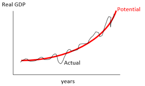
Figure 8.1 has good news and bad news. The good news is growth—over time, real GDP has increased, and the curved nature of the path portends big increases in the future. Figuring out how the market system delivers such growth in output over time remains a central unsolved problem in economics.
The bad news is the fluctuations in output—every drop in actual real GDP causes pain via job loss and firm collapse. Understanding why the market system is so erratic is another central unsolved problem in economics.
These two fundamental properties of market economies, long-run growth and short-run fluctuations, drive the organizational structure of macroeconomics. For long-run analysis, we use growth theory models and focus on the trend of real GDP per person with a time scale of decades or more. An important goal is to make output per person grow fast, with 2% per year considered very good for rich countries. Seemingly small percentage point increases in CAGR produce huge gains over long periods of time.
Short-run macroeconomics pays little attention to population growth, since it remains roughly the same from one quarter to the next, and focuses on explanations for rising and falling GDP from one quarter to the next. Instead of CAGR over many years, the most common measure is the annualized percentage change in GDP from one time period to the next. When positive, the economy is booming, while negative percentage changes indicate recession.
In the short run, more variables come into play, such as prices, interest rates, and future expectations, because they seem to impact the boom-bust cycle. A key goal is to stabilize the economy. Government policy makers actively attempt to manipulate the economy so as to even out the variability and reverse downturns. We want not only acceleration but a smooth ride.
Figure 8.1 is not based on actual data, but the roller coaster or boom-bust depiction is a feature of the market system. Figuring out why the economy roars and then stagnates is one of the central questions in short-run macroeconomics.
STEP Insert a new sheet in your workbook and use FRED to get data on GDPPOT and GDPC1. Make a single chart (use an initial date of 1/1/1950 for GDPC1) of both series.
Unlike Figure 8.1, your chart shows that the US economy has been above its path (potential GDP) for a while. This is certainly welcome news and will influence future projections of potential output. The Great Recession of 2008 and the effects of the COVID-19 pandemic are clearly visible.
You may have noticed that we used GDPC1 instead of GDP (as in the previous section). The difference between the two is how they incorporate prices. GDPC1 is real GDP and GDP (without the C1) is nominal GDP.
Real GDP holds prices constant, so its changes are due solely to output changes. Nominal GDP uses current prices, so its changes are a combination of output and price changes.
GDPC1 uses chained dollars (hence the C) to hold prices constant. Because buyers respond to changing prices and innovation creates new products, it is impossible to maintain a truly fixed basket of items with which to construct a price index. Chained dollars are a way around this problem, and they are used for many other macro variables—whenever you see “chained dollars,” that means the variable has prices held constant and is in real terms.
Real GDP is the correct GDP to use when you are interested in how the economy is doing over time. If you use nominal GDP and there is inflation, you might conclude that the economy is growing rapidly when it is just rising prices making nominal GDP increase.
Who’s Responsible?
Let’s dive down into real GDP and explore its components. Our goal is to see if we can figure out why real GDP is so volatile. Is it C, I, or G? In other words, are consumers, firms, or governments responsible for the business cycle?
This is not a mystery novel, but we like surprises, so we will wait for the big reveal. You might want to pick one and see if you get it right.
STEP Insert a new sheet in your workbook and enter GDPC1, PCECC96, GPDIC1, and GCEC1 in the first row. Enter pca in the second row (under each SERIES ID). Get the data.
You are looking at the annualized percentage change (that is what pca does) for each macro aggregate. We need to visualize the data to understand what is going on. We start with real GDP.
STEP Use FRED’s charting tool to make a graph of annualized percentage changes in GDPC1 over time.
Figure 8.2 shows what your chart should look like. There are two things to notice. First, the percentage change is negative in every recession. This makes sense, since the definition of a recession is a downturn in the economy. Second, before 1980, it seems the economy was more volatile than after 1980. Look carefully at how the spikes hit and exceed 10.0 percentage points before 1980, but they are more tamped down after the recession in the early 1980s.
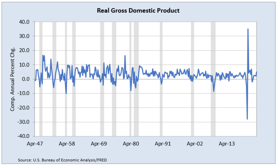
Source: U.S. Bureau of Economic Analysis via FRED, Public Domain Data / FRED Terms.
So which of the three macro aggregates—C, I or G—is responsible for this? You get one last chance to guess before the big reveal.
STEP Create three individual charts of C, I and G. Stack them on top of each other.
At first, they seem similar, but look carefully at the y-axis of each chart. We need to standardize them to compare them correctly.
STEP Change the y-axis min and max to −100 and 150 in the C and G charts so that the three charts have the same y-axis.
The result is dramatic. It is easy to see that investment is much more volatile than consumption or government spending.
STEP Another way is to create a single chart with C, I, and G. Use FRED’s Create Multiple Series Graph to do this.
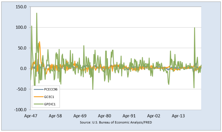
Source: U.S. Bureau of Economic Analysis via FRED, Public Domain Data / FRED Terms.
Your chart (the same as Figure 8.3) clearly shows investment volatility swamping consumption and government spending. It is not that C and G do not matter—in fact, a great deal of effort is devoted to explaining how C changes. Forecasting consumer sentiment and spending is important.
But there is no question that a critical source of the volatility in GDP is coming from I. The question then becomes, Why is investment so volatile?
We know investment depends on interest rates from our previous work on IRR. For a project to be undertaken, the IRR must be greater than the appropriate discount rate. Often, this is a cost of funds measure or market interest rate. Thus, as interest rates fall, investment rises and vice versa.
Thus, conventional wisdom says that investment is volatile because interest rates bounce around a lot. But there is another important factor affecting investment: emotion.
John Maynard Keynes, the leading economist of the first half of the 20th century, argued that interest rates alone could not explain the volatility of investment. He coined the term animal spirits to capture the instinctual and primitive forces that help drive decision-making:
Even apart from the instability due to speculation, there is the instability due to the characteristic of human nature that a large proportion of our positive activities depend on spontaneous optimism rather than on a mathematical expectation, whether moral or hedonistic or economic. Most, probably, of our decisions to do something positive, the full consequences of which will be drawn out over many days to come, can only be taken as a result of animal spirits—of a spontaneous urge to action rather than inaction, and not as the outcome of a weighted average of quantitative benefits multiplied by quantitative probabilities. Enterprise only pretends to itself to be mainly actuated by the statements in its own prospectus, however candid and sincere. Only a little more than an expedition to the South Pole, is it based on an exact calculation of benefits to come. Thus if the animal spirits are dimmed and the spontaneous optimism falters, leaving us to depend on nothing but a mathematical expectation, enterprise will fade and die;—though fears of loss may have a basis no more reasonable than hopes of profit had before.[1]
Keynes was a genius and polymath. He managed the portfolio at King’s College (one of Cambridge University’s wealthiest colleges), where he was a professor. He knew philosophy and art but also understood mathematics and what we call today analytics. He was convinced that human behavior had a subjective element that required going beyond data. He was an early behavioral economist who was interested in the psychology of individual and group decision-making. Keynes did not believe that we could explain the volatility of investment with interest rates alone. Animal spirits captured the instinctive, nonquantifiable, irrational forces that drive us.
There is no doubt about it: Investment is the source of the volatility in GDP. Investment is driving the business cycle. Figuring out how and why I is so volatile is at the top of the research agenda in modern short-run macroeconomics.
Takeaways
The key equation in national income accounting is
GDP = C + I + G + NX.
This says that total output can be measured by adding the spending of consumers, firms, and governments (with an adjustment for net exports).
National income accounting is all about categories and adding up subcategories into bigger aggregates. Investment, for example, is composed of spending by firms on new tools, plant, and equipment, plus new housing construction, plus changes in business inventories (a subcategory to handle goods sold in a later time period).
Long-run macroeconomics is about the path the economy is on, while short-run analysis focuses on the ups and downs of the business cycle.
Instead of computing a CAGR over long periods of time, the short run is about quarterly changes or predicting how the economy will be doing a few months from now.
A core question in the short run concerns the intense volatility of market economies. Booms are followed by busts in a wild roller coaster ride. The focus is on identifying the source of the volatility and how to manage it.
Investment is the culprit. It has much bigger ups and downs than C or G.
While interest rate movements contribute to investment fluctuations, animal spirits (defined by Keynes as a “spontaneous urge to action”) often produce waves of euphoria and rapid upswings in the economy that are then followed by pessimism and recession.
If you want to see Keynes speaking from a 1930s newsreel and learn more about his most famous book, The General Theory of Employment, Interest and Money, visit vimeo.com/200367754.
References
The epigraph is from pp. 1–2 of “Concepts and Methods of the U.S. National Income and Product Accounts” (visited in November 2023 and available at www.bea.gov/methodologies/index.htm#nationalmeth). This document answers the question, How did the NIPAs originate? It is noteworthy that the person instrumental in setting up British national income accounts, Richard Stone, also received a Nobel Prize in Economic Sciences. Establishing a coherent, reliable methodology for aggregate measures of economic performance is not trivial.
Keynes, J. M. (1936). The General Theory of Employment, Interest and Money. Full text online at www.marxists.org/reference/subject/economics/keynes/general-theory.
U.S. Bureau of Economic Analysis, Real Gross Domestic Product [GDPC1], retrieved from FRED, Federal Reserve Bank of St. Louis; https://fred.stlouisfed.org/series/GDPC1.
U.S. Bureau of Economic Analysis, Real Gross Private Domestic Investment [GPDIC1], retrieved from FRED, Federal Reserve Bank of St. Louis; https://fred.stlouisfed.org/series/GPDIC1.
U.S. Bureau of Economic Analysis, Real Government Consumption Expenditures and Gross Investment [GCEC1], retrieved from FRED, Federal Reserve Bank of St. Louis; https://fred.stlouisfed.org/series/GCEC1.
U.S. Bureau of Economic Analysis, Real Personal Consumption Expenditures [PCECC96], retrieved from FRED, Federal Reserve Bank of St. Louis; https://fred.stlouisfed.org/series/PCECC96.
For a more modern take on the role of psychology in investment and human behavior, see Akerlof, G., and Shiller, R. (2010). Animal Spirits: How Human Psychology Drives the Economy, and Why It Matters for Global Capitalism (Princeton University Press).
8.2 International Comparisons
We know that national income accounting is grounded on this key equation:
GDP = C + I + G + NX.
Simple logic says that fluctuations in GDP must depend on its components, and the data for the United States show that investment is more volatile than consumption and government spending.
But what about other countries? Is investment responsible for the boom-and-bust nature of GDP in other economies?
Data from the Organisation for Economic Co-Operation and Development (OECD) answer this question. This international agency was created after World War II and serves, in part, as a hub for data gathered from member countries. They are online at oecd.org, but we will access the data through the FRED Excel add-in.
There is a data issue to address before we explore the volatility of investment in other countries. Instead of investment spending, the OECD reports gross fixed capital formation (GFCF) as a measure of investment activity.
There are several differences between I and GFCF, but the key one is that GFCF includes secondhand assets (think of used heavy machinery that is purchased by a manufacturing company). Investment, on the other hand, counts only new tools, plant, and equipment.
STEP Insert a sheet in your GDPInvestment.xlsx workbook. In the top row, enter GPDIC1 (this is real I) and NAEXKP04USQ652S (this is real GFCF). Enter 01/01/1972 in cell A4 (so both series start from the same date) and get the data. Widen column D if needed.
Investment spending is in billions of dollars, so to make it easier to compare the two, we need to convert GFCF to billions of dollars.
STEP Enter the formula =D8/1000000000 (carefully enter 9 zeroes) in cell E8. Fill it down.
It is easy to see that column E, GFCF (in billions), is greater than column B (I in billions). This is mainly because GFCF counts the resale of previously produced tools, plant, and equipment, and I does not. It also means that you would not get C + GFCF + G + NX to equal GDP.
It is not that GFCF is wrong, but we want to be aware that it is a different measure of investment activity than I. The OECD uses GFCF in its country reports and highlights it as their preferred measure of investment activity. We will compare the volatility of GFCF to C and G to answer our question.
OECD Countries and Series IDs
The OECD has data on real C, GFCF, and G for 39 countries. We will focus on the major economies in the OECD, called the G7: Canada, France, Germany, Italy, Japan, the United Kingdom, and the United States.
To get the data, we parse the Series ID we used to get GFCF for the United States: NAEXKP04USQ652S. To parse means “to separate something into its component parts.”
The Series ID for OECD macro aggregates has five parts. We can show this using vertical line separators:
NAEXKP|04|US|Q|652S.
In the second part, the 04 indicates GFCF; 01 is GDP, 02 is C, and 03 is G.
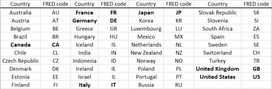
The third part is a two-character country code. The table in Figure 8.4 shows the two-letter abbreviation for each country.
The last part is troublesome because it is different for different countries. This means that we cannot simply plug in the two-letter FRED code for each country because the last part of the Series ID (the part after the Q) is not always the same. As a work-around, we use FRED’s search tool.
STEP Insert a sheet in your GDPInvestment.xlsx workbook and click the Data Search button. In the search box, enter the text NAEXKP02USQ and click the Series ID option (below the search box). Click the Search button. Select the series with units of US $ and click the Add Series IDs button at the bottom of the dialog box. Change the 2 to a 3 in the search box and repeat the procedure: search, select the series with units of US $, and add it to the spreadsheet. Change the 3 to a 4 and repeat again. Click Close and then get the data.
You have real C, G, and GFCF for the United States. But we want the annualized growth rate for each quarter, and we want to start from the same date.
STEP Change lin to pca in each cell in row 2, and set the start date in row 4 to 04/01/2002 (since that is the latest date for the series). Get the data.
We are ready to answer the question of which component is the most volatile for the United States, but this time using GFCF instead of I.
STEP Use FRED’s Build Graph tool to put the three series on the same chart.
GFCF seems a little more variable than C and G, but the difference is not as dramatic as when we used investment spending. Also, there is a sharp increase in G in 2007 that is not in the NIPA data. That is an error in the OECD data.
The SD
Before we explore the other G7 countries, we offer a more objective measure with which to gauge volatility than the eyeball test we have been using.
The standard deviation, or SD, is a measure of dispersion in a list of numbers. if the numbers are bunched tightly together, the SD is low (if they are all the same, then the SD is zero). The more spread out the numbers, the larger the SD.
The SD has the same units as the numbers. If we measure the heights of 20 college students in inches, then the SD is in inches.
Think of the SD as a +/− number. The SD tells us the size of the typical deviation from the average. If the average height is 5 feet, 8 inches with an SD of 3 inches, that says most of the students are around 5 feet, 8 inches tall, give or take 3 inches. In other words, most of them are between 5 feet, 5 inches and 5 feet, 11 inches.
It would not make sense if the SD of the height of 20 college students was 4 feet, because then the range is from under 2 feet to almost 10 feet tall.
STEP Return to the sheet with GDP, C, I, and G (from the US NIPAs) and scroll down to the bottom row. In any row after the last row, in column B, use Excel’s STDEV.P function to compute the SD of real GDP. Copy your formula and paste it in columns D, F, and H.
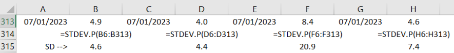
Figure 8.5 shows the result as of fall 2023 (so 07/01/2023 is the last value). Investment spending is in column F, and it has a much higher SD, or dispersion, than C or G. Does the same hold true for GFCF?
STEP Return to the sheet with the OECD measures of C, G, and GFCF. Scroll to the bottom and compute the SDs for the three series. Yes, GFCF has a higher SD than C or G, but not by a lot.
Discovery
What about the other G7 countries? Use the same steps applied to the United States to explore the volatility of C, G, and GFCF in the other G7 countries.
STEP Download OECD data on the annualized percentage change in real C, G, and GFCF. Make a chart. Compute the SDs of the three series. What do you find with respect to the crucial question about volatility in GDP—is investment driving volatility in GDP for these economies?
Notice that the Series IDs can be tricky to work with in this case. Confirm that the Series IDs are correct and that they make sense. It is easy to make a mistake. A simple check is to click on the URL in row 5 of each variable and make sure it is the correct country and series.
- Source: Keynes (1936, chap. 12) ↵
