
3 Leverage Data Visualizations to Show Trends and Insights
It is true that data visualization is part data science and part art. That being said, even the most creative art is supported by theories that explain why it works.
—Michiko I. Wolcott, CMC, 20-year veteran of consulting in data and analytics
What Do You Think?
Sarah, a marketing executive, is eager to present data findings to her VP, but struggles to interpret and communicate them effectively. Sarah has invited her colleague, Alex, to give the presentation. Alex is passionate about uncovering trends through data visualization. Any time a question comes up about working with the company’s data, Sarah is always told, “Go ask Alex.” Sarah forwarded her last year’s data to Alex and scheduled a virtual conference call.
As Sarah joins the meeting, she is met with a complicated data visualization shared on her screen. Before she can even say “hello,” Alex exclaims, “Sarah, I’ve spent hours analyzing the data, and I believe I’ve found some incredible trends that can help drive next year’s marketing strategy!”
Sarah looks at the visualization and nervously responds, “That’s great, Alex! But I must admit, this data visualization seems a little overwhelming. How can we simplify it for our presentation?” Alex turns on his camera, “I understand your concern, Sarah. We need to find a way to break down the complexity and present the trends in a clear and concise manner. How about we focus on the key insights and simplify the visualization to make it more understandable?”
Sarah, with a sigh of relief, responds, “Thanks, Alex, I like this plan! So what were the most significant trends discovered?”
Alex leans in, “Well, one trend that stands out is the correlation between our social media campaigns and website traffic. There is a substantial increase in website visits following each campaign launch.”
Alex smiles and responds, “Let’s use a line chart to showcase the website traffic over time, with clear markers indicating the dates of each social media campaign. This way, we can demonstrate the direct impact of our campaigns on generating traffic!”
Alex sees Sarah taking notes. She looks up, and he can see her excitement as she responds, “I can already visualize it. And I know the perfect story to include—we have a great testimonial from a customer about our July campaign to go with it. What other trends have you found?”
Alex showed Sarah three more insightful trends. The collaborative nature of their discussion heightened their determination to deliver a compelling and informative story with insightful data visualizations.
In this scenario, Alex and Sarah faced the challenge of presenting a complex data visualization that shows trends. Think about your own organization. Do you look for insight from your data to strategize goals for next year?
Introduction
In the age of information overload, harnessing the power of data has become paramount for organizations seeking a competitive edge. In the scenario, Sarah recognized the ability to extract meaningful trends and insights from complex datasets was a skill she needed—a skill that can translate into a strategic advantage. Alex was able to transform the raw data and suggest visuals, but it was Sarah who saw a need to incorporate a story. As they collaborated on visual narratives that would bring data to life, they brainstormed ways to make them more accessible (easier to understand) and engaging for their main decision-maker, their VP.
Within this chapter, we will delve into the principles and best practices of leveraging data visualizations to unveil trends and insights. We will explore various visualization techniques and tools, highlighting their strengths and applications in different contexts. Graphical displays of data make it easier to spot patterns and detect unusual values. Besides the graphical displays to help us understand our data, this chapter also introduces benchmarking, tools used to visualize and persuade, statistical analysis tools, and visuals to support decision-making.
We will also explore techniques to effectively communicate insights derived from data visualizations for diverse audiences, ensuring that the impact of the findings is maximized. So let’s embark on a journey to leverage data visualizations, unravel the hidden stories within the data, and uncover trends and insights that can shape the future of our organizations.
Chapter 3 addresses the following learning objectives.
Learning Objectives
At the end of this chapter, students should be able to:
- LO 1: Determine insights.
- LO 2: Use benchmarking, decision-making, and strategic analysis tools.
- LO 3: Interpret research industry trends and recognize bias.
- LO 4: Create and use benchmarking frameworks to provide context for problems, support decisions, and measure performance.
- LO 5: Create and use decision-making tools to provide context for problems, support decisions, and assess risk.
- LO 6: Conduct preliminary statistical analysis, predictive statistics, and understand Six Sigma.
Key Terms: Balanced Scorecard, decision trees, descriptive statistics, Disruptor, Ishikawa, MarketLine, Pareto Diagrams, PEST, PESTLE, Porter’s Five Forces, posters, regression analysis, Six Sigma, sparklines, SWOT
3.1 An Introduction to Anscombe’s Four Datasets
The goal is to turn data into information and information into insight.
—Carly Fiorina, former CEO of Hewlett-Packard
One of the best ways to see the importance of making a visual of data is to introduce the Anscombe datasets. In 1973, Anscombe built four datasets of 11 points each. Statistically they are very similar: Averages, variances, correlation, and even the linear regression formula are the same. Here are the four datasets slightly modified from the original. The modifications are highlighted in Figure 3.1.
Figure 3.1—Modified Anscombe’s Quartet
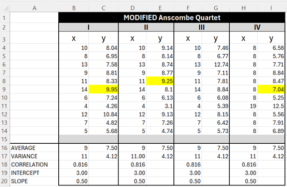
Note: The yellow highlighting are numbers that are slightly different from the original Anscombe’s quartet dataset.
When calculated, the following statistical information is true for each of the four datasets.
- The average x value is 9; the average y value is 7.50.
- The variance for x is 11 and the variance for y is 4.12.
- The correlation between x and y is .816.
- The linear regression is y = .50x + 3.
Figure 3.2—Formulas in Excel: Using Dataset I as an Example
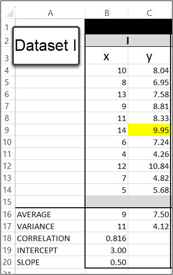
To calculate the average (arithmetic mean) for Dataset I, use the formulas
=AVERAGE(B4:B14)
and
=AVERAGE(C4:C14).
To calculate the variance (measures the spread) for Dataset I, use the formula
=VAR(B4:B14)=VAR(C4:C14).
To calculate the correlation (measures the relationship between x and y) for Dataset I, use the formula =CORREL(B4:B14,C4:C14). The .816 is the correlation coefficient. A value of 1 means a perfect positive relationship. A value of 0 means no relationship, and a value of −1 means a perfect negative relationship. Correlation tells you the degree (or strength) to which two variables move in relation to each other. Correlation measures association but not causation. In data analysis, you will see correlation as one of the statistical methods. The correlation (R) is not the same thing as R Square (R2). R Square is the coefficient of determination and tells you how many points fall on the regression line.
To calculate the intercept at the y-axis in regression for Dataset I, use the formula = INTERCEPT(C4:C14,B4:B14). I like the name intercept, because it tells you where it will cross the y-axis. You will also see mathematicians refer to this as alpha.
To calculate the slope of regression for Dataset I, use the formula =SLOPE(C4:C14,B4:B14). You will also see mathematicians refer to this as beta.
Regression line (y = 3 + .50x) with a goodness of fit at .816.
Think of a regression line where y = a + b(x). x is the explanatory variable, and y is the dependent variable. The slope of the line is b, and a is the intercept on the y-axis.
A Scatterplot in Excel
A scatterplot displays values for two variables and is often used to investigate the relationship between two variables. A scatterplot can show a positive relationship, a negative relationship, or no relationship at all. A positive relationship (uphill pattern from left to right) means that as one variable increases, the other variable also tends to increase. A negative relationship (downhill pattern from left to right) means that as one variable increases, the other variable tends to decrease. If there is no relationship, there will be no clear pattern. Let’s look at the scatterplot graphs for the four datasets in Figure 3.3.
Figure 3.3—Scatterplots of the Anscombe’s Quartet
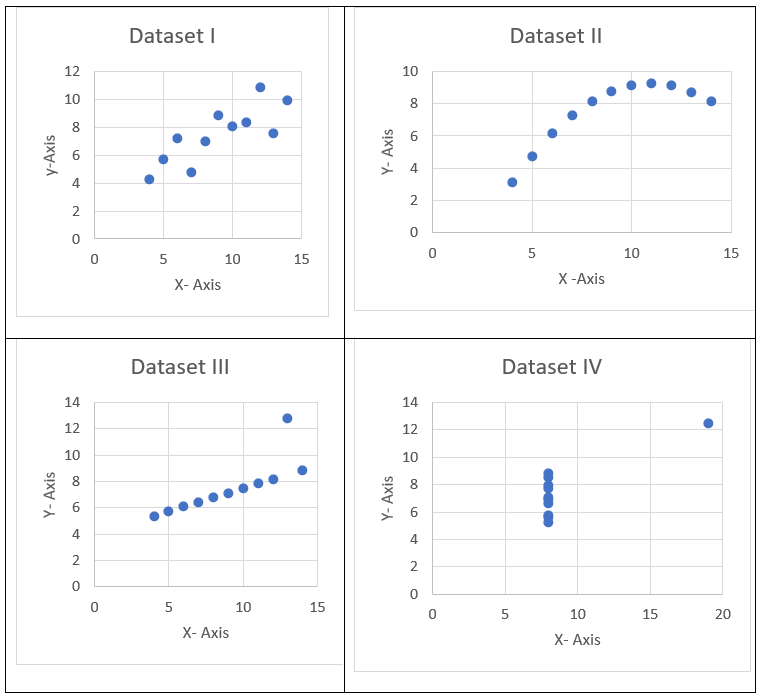
Keep in mind that all four datasets have the same average, variance, correlation, intercept, and slope.
As you can see from Figure 3.4, the average, variance, correlation, and intercept are the same.
Figure 3.4—Anscombe’s Quartet Comparison
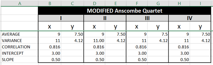
The average, variance, correlation, intercept, and slope calculated in Figure 3.4 would lead a researcher to think that each dataset would graph the same. Despite the similarities, we see very different graphs.
- In Dataset I, we see a set of points that appear to follow a roughly linear relationship with some variance.
- In Dataset II, we see a clear curve with no linear relationship (perhaps quadratic).
- In Dataset III, we see a tight linear relationship with one outlier.
- In Dataset IV, x appears to remain constant with one outlier.
This exercise supports the importance of visualization. You may want to explore the Excel file and look at each dataset. The average, variance, correlation, intercept, and slope formulas are calculated under each dataset, but you can also explore the linear regression completed for each dataset. Regression will be explained and explored later in this chapter.
 Anscombe, F. J. (1973). Graphs in Statistical Analysis. The American Statistician. Vol 27. Issue 1 p. 17–21.
![]() Mitchell, J. (2021, Apr 9). Scatter plot in Excel and SPSS Version 27. [Video]. YouTube.
Mitchell, J. (2021, Apr 9). Scatter plot in Excel and SPSS Version 27. [Video]. YouTube.

This dataset is available for this chapter in Excel.
 Step-by-Step—Create a Scatterplot in Excel for Dataset I
Note: Screenshots of Excel interface © Microsoft Corporation, used with attribution for instructional and illustrative purposes. Annotations added by the author.
- Open the “Chapter 3-Anscombe Quartet-Adj” data file and go to the tab Anscombe Quartet-Adj.
- Highlight the X and Y columns of Dataset I (this is B4:C14).
- On the insert menu, choose the chart icon that resembles a scatterplot and choose scatter as shown in Figure 3.5.
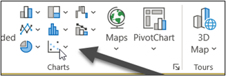
Figure 3.5—Scatterplot Chart Icons The graph (shown in Figure 3.6) will need further work. It needs a title (e.g., Dataset I) and axis titles to label the x-axis (horizontal) and the y-axis (vertical).
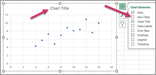
Figure 3.6—Draft Scatterplot Chart - The final graph shows a positive correlation, titles, bolded values, and even a trendline! This graph (Figure 3.7) demonstrates a positive correlation (as x increases, so does y).
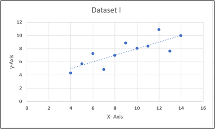
Figure 3.7—Scatterplot of Dataset 1 With Trends
Real-Life Example of an Impactful Scatterplot
Prior to 2010, estimating the age of unidentified crime victims was done by examining teeth and bones. A groundbreaking study, Estimating Human Age From T0Cell DNA Rearrangements, was conducted in 2010 by examining the age and blood test measure. The study included 195 people ranging in age from a few weeks to 80 years old.
Please visit:
Zubakov et al. (2010). Estimating human age from T-cell DNA rearrangements. Current Biology Vol 20 #22. https://www.cell.com/action/showPdf?pii=S0960-9822%2810%2901286-8
- R2 = 0.835 and means that approximately 83.5% of the variability in age can be explained by the linear relationship between age and blood test measure.
- alpha = −33.65 is the y-intercept (note this is negative).
- beta = −6.74 is the slope (note this is negative).
- Equation: The linear equation is y = −33.65 − 6.74(x), so as a crime investigator, a victim with a blood sample of −11 would mean the age of the victim is 40.49 calculated as ŷ = −33.65 − 6.74(−11) = 40.49 years
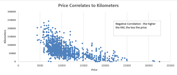
Correlations can be positive or negative. Let’s look at a negative correlation of a single brand of car and how price correlates to the number of kilometers. It makes sense that the more kilometers on the car, the less the price. See Figure 3.8a.
Figure 3.8a—Negative Correlation – Scatterplot of Age of Car Compared to Price
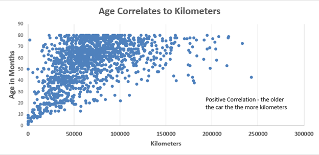
If we were to compare the car’s kilometers to the age of the car, we would see a positive correlation as shown in Figure 3.8b.
Figure 3.8b—Positive Correlation – Scatterplot of Age of Car Compared to Kilometers
3.1 Self-Assessment Insights of Anscombe
Learning Objective #1—Determine insights

3.1 Exercise 1: Discussing Terms Used in Anscombe’s Quartet
Learning Objective #1 Determine insights
 Your company requires all employees to complete a training series on culture. Everyone has access to the same online training conducted by a third party. Individuals can spend as little or as much time as they need, since employees may rewatch videos or revisit content. At the end of the series, every employee takes an online exam. After completing the training, the third-party vendor provides the following information to HR as shown in Figure 3.9. The vendor indicates that most employees would only need to spend seven hours to earn a passing grade of 70%.
Figure 3.9—Training Datasets
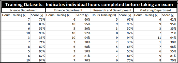
This report is available in the Chapter 3 Excel file.
Your supervisor has asked you to analyze this data for insights.
- What are the averages, variances, correlation, intercept, and slope?
- Using the regression formula y = a + b(x), what score should you earn if you spend 7 hours in training depending on the department?
- Does this report agree with the vendor’s claim that individuals who study 7 hours will pass the exam? Create scatterplot graphs. Which one is close to the trend line?
- Present your findings, including your Excel sheet, either in class or on the bulletin board as directed by your instructor.
3.2 The Simplest Graphics—Sparklines, Icon Arrays, Combo Charts, and Word Clouds
The art of data visualization lies in capturing the essence of trends, distilling complexity into simplicity, and enabling minds to grasp the pulse of change.
—Anonymous
What are sparklines? Sparklines are small, condensed visual representations of data that are great for a quick overview of trends and patterns. They are not detailed like full-fledged charts or graphs, but they offer several insights. They are so tiny that they fit within one cell of a spreadsheet!
The easiest way to understand these is to see an example, so let’s look at POM University ticket gross revenue and ticket net income for 2010 through 2023, shown in Exhibit 3.1. Note how the sparklines show the trend all from within one cell for each row.
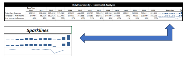
POM University’s gross revenue and ticket sale net income between 2010 and 2023 show a healthy rise of income and net income until 2020–2021 (during COVID-19). The sparklines show the trend of the gross revenue and net income as well as the horizontal analysis.
There are three different types of sparklines: line, column, and win/loss.
Perhaps as you review the sparkline, you might ask “What about the percentage of income to revenue?” In 2010, we see a 40% profit margin, which increased to 51% in 2016. However, the percentage dropped in the COVID-19 years and has still not reached baseline (2010) performance. How can you bring these details to the attention of your audience? One way would be to combine graph types using a combo graph; but first, let’s show the step-by-step process to create sparklines.
Step-by-Step Approach to Create a Sparkline in Microsoft Excel
Note: Screenshots of Excel interface © Microsoft Corporation, used with attribution for instructional and illustrative purposes. Annotations added by the author.
- Prepare your data. Open an Excel document and type in the months and revenue data shown in Figure 3.10.
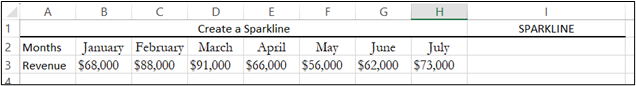
Figure 3.10—Excel Data for Sparkline Chart - Select the cell where you want to insert the sparkline (in this case, cell I3).
- Go to the Insert tab in the ribbon.
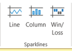
- Click on the Sparklines button in the Chart group. A drop-down menu will appear with the three types of sparklines (as illustrated in Figure 3.11). Choose the Line chart to show the revenue trend.
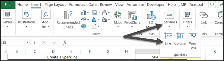
Figure 3.11—Sparklines - Once you choose a sparkline, a window will pop up for the data range (B3:H3) and the location range (see Figure 3.12). Then click OK and see your sparkline. Try each type so you can see how they chart.
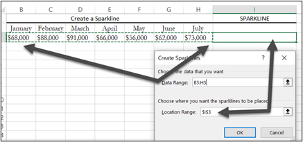
Figure 3.12—Create a Sparkline for Revenue - Customize the sparkline by clicking on the sparkline in cell I3 as shown in Figure 3.13. This will add an extra tab Sparkline on the main menu If you choose it, you will see lots of design and format options.
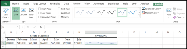
Figure 3.13—Customize the Sparkline
With sparklines, you can identify trends including seasonal patterns or volatility. They offer a quick visual cue. Now let’s talk about a slightly more interesting graph, an icon array.
Using Icon Arrays
An icon array uses small symbols to represent individual data points. They are useful for frequencies or proportions. Figure 3.14 shows an example created in Venngage (see Chapter 2). There are specific uses of color, specific icons, and color coordination of the icons.
Figure 3.14—Icon Array Example Using Venngage
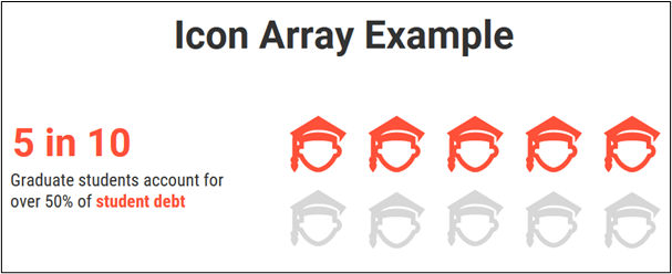
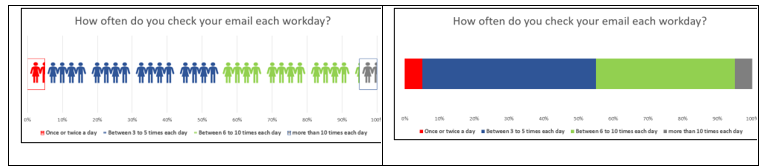
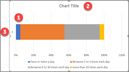
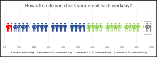
Exhibit 3.2 shows an example of starting with a horizontal stacked bar chart often used to represent the results of survey questions. In this example, instead of bars, you see icons representing the results. Notice that the colors also represent information to the viewer. Red represents concern, and gray represents a “gray area” where employees check their email too often.
Exhibit 3.2—Icons in a Horizontal Stacked Bar Chart—a Comparison
Try your hand at creating an icon chart in this step-by-step approach.
Step-by-Step Approach to Create an Icon Array in Excel: Adding Icons to a Horizontal Stacked Bar Chart
Note: Screenshots of Excel interface © Microsoft Corporation, used with attribution for instructional and illustrative purposes. Annotations added by the author.
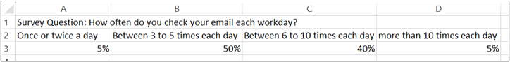
1. Let’s start with some simple survey results that were collected at an organization. Essentially, the survey question was “How often do you check your email each workday?”
The summarized results of the survey: 5% checked their email once or twice each day; 50% checked their email between 3 and 5 times each day; 40% checked their email 6 to 10 times each day; and 5% checked their email more than 10 times each day. Set up your Excel sheet as shown in Figure 3.15 (or use the Excel workbook for Chapter 3).
2. Highlight A2:D3 and choose Insert on the main menu and then column or bar chart.
3. Scroll down to “More column charts” and choose Bar and select the stacked bar chart (as illustrated in Figure 3.16).
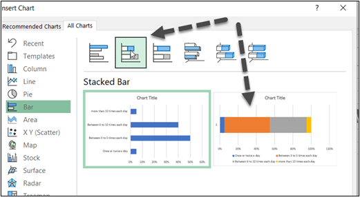
4. Select OK.
5. Customize: The chart, as illustrated in Figure 3.17, needs customization to reflect the following colors, add a title, and clean up the axis titles.
![]() Right-click on the color you wish to change. Choose Format Chart Area and change color to show red, yellow, green, and gray. Use these colors to take advantage of the audience’s understanding of traffic lights (red, yellow, and green).
Right-click on the color you wish to change. Choose Format Chart Area and change color to show red, yellow, green, and gray. Use these colors to take advantage of the audience’s understanding of traffic lights (red, yellow, and green).
![]() Change the chart title to How often do you check your email each workday? Further customize it to bold and larger font.
Change the chart title to How often do you check your email each workday? Further customize it to bold and larger font.
![]() Remove axis titles if present. Feel free to further customize the legend. Make sure the legend colors match the new colors. The stacked bar chart is the most commonly used chart for survey data. If you wish to make a bold statement, add the 50% and 40%, especially if these two categories of responsiveness are within the organization’s policy about checking email.
Remove axis titles if present. Feel free to further customize the legend. Make sure the legend colors match the new colors. The stacked bar chart is the most commonly used chart for survey data. If you wish to make a bold statement, add the 50% and 40%, especially if these two categories of responsiveness are within the organization’s policy about checking email.
![Horizontal stacked bar chart titled "How often do you check your email each workday?" with 50% on the section for "Between 3 to 5 times," and 40% on "Between 6 to 10 times." [3.13b shows the same info with an icon array.]](https://pressbooks.palni.org/leveragingdatavisualizationtocommunicateeffectively/wp-content/uploads/sites/54/2025/03/fig0318.png)

6. Add an icon array. We could stop here, or we could change the chart to show icons. If you pick the icon from those available, they are easier to match to the colors.
a. Go to Insert on the main menu, then Illustrations and choose Icons.
b. Type “people” in the search bar.
c. Choose an icon that shows people. And then click OK. For this example, choose the icon that looks like male and female figures.

d. When it copies to Excel, you will notice that the image should be cropped. To crop the image, right-click the image and choose Format Graphic, then choose the icon that looks like a mountain as shown in Figure 3.21. Then use “crop position” to crop the height to .70″ and top to 1.1″ If these do not work for you, try adjusting them slightly. The others can remain at their default.

e. Color the icon red to match. Right-click the the icon, choose Format Graphic, and color it the same red as what you see on the stacked horizontal bar. It looks like Figure 3.22.
f. Now use a keyboard shortcut (Ctrl + c) to copy the people, select the first red bar of color, and use (Ctrl + v) to paste to the block.

When you do, the people will look squeezed together as shown in Figure 3.23.
g. Make sure you have the squeezed-together people highlighted, right-click, then select Format Data Point, then choose the paint bucket icon, then Stack. When you do, you will see the images fill it properly.

h. Just follow steps e–g for the next bars. (Note that the next bar is blue now instead of yellow. That’s because the yellow icons were difficult to detect.) Your final product should look like Figure 3.24.
Assessing the Effectiveness of an Icon Array
People-First Language: Be careful when you use icons to represent specific people. Use person-first and identity-first language. Instead of “a cancer patient,” use “a patient with cancer.” Instead of “AIDS patients,” use “people with AIDS.” The goal is to avoid language that dehumanizes or stigmatizes people. It is recommended to review any infographic or icon array with this perspective in mind.
Accessibility: Ensure that the icon array is accessible to individuals with disabilities like visual impairment or even audience members who are color-blind.
There are five main ways to assess the data visualization known as an icon array. These include the following:
- Accuracy and clarity: Do the icons use consistent size, shape, and color? Does it accurately represent the data? Can the audience easily understand what each icon represents?
- Perceptions and comprehension: For this aspect, conduct user testing with similar people who will make up the audience. Are people able to accurately interpret the data values and trends being displayed? For example, using people icons may send mixed messages when colors are introduced.
- Comparison and contrast: Can viewers easily identify differences in the data values represented by the icons? Are they able to compare values across different categories or groups?
- Scalability and density: Can the visualization handle a large dataset without becoming overcrowded or losing clarity?
- Engagement and memorability: Does the visualization capture the audience’s attention and encourage further investigation into the topic? Does the audience remember the visualization weeks after seeing it?
Working With a Horizontal Stacked Bar Chart
Before we move away from horizontal stacked bar charts, let’s review a few tips and tricks. Most researchers use some type of software to create a survey like Survey Monkey, JotForm, Qualtrics, Google Forms, Lime Survey, and so on. Most survey software will allow you to export to Excel; however, moving beyond the basic charts can improve data storytelling. Horizontal stacked bar charts are useful for visualizing data that involves multiple categories as well as proportions and their relationships.
For example, a horizontal stacked bar chart can be used to
- display the different types of expenses in a budget for various departments or display or showcase resources (time, budget, personnel).
- display a summary of the different survey responses including a further subcategory (like demographic groups).
- display a summary of pretest and posttest survey results. This is especially helpful to compare a before and after survey, like Figure 3.25 of students who took a precourse and postcourse survey.
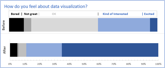
Figure 3.25—Example of a Horizontal Stacked Bar Showing Before and After Survey - display a project timeline by representing the progression of tasks over time.
- display educational assessment through a distribution of grades across various categories.
In the realm of data visualization, concise and effective techniques offer invaluable insights into complex datasets. At one end of the spectrum, sparklines show powerful trends for a quick overview of data patterns over time. Icon arrays, with their adept use of symbols, deliver an intuitive representation of proportions and frequencies, making them ideal for visualizing categorical data. Horizontal stacked bar charts work great for survey questions. But as we venture deeper into the visualization landscape, the true versatility of combining these techniques comes to light with combo charts. These hybrid visualizations merge multiple graph types into a single cohesive display, presenting a wealth of information at a glance.
What Is a Combo Graph?
A combo graph (or combo chart) is a combination of two bar charts, two line graphs, or a bar chart and a line graph(s). You can work from a single dataset or two datasets as long as the datasets share a common base. You want to use combo graphs to show some kind of relationship or trend.
Example 1—Combo Chart With One Bar Chart and One Line Graph
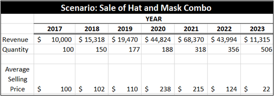
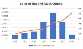
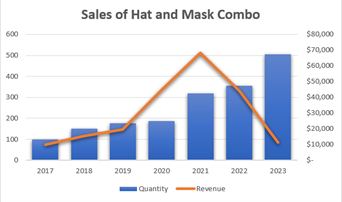
Consider a scenario where you want to analyze the sales performance of a product over time. Using a combo chart to combine a bar chart and line graph allows the viewer to easily depict the relationship between revenue and quantity trends. It shows the audience if a lower revenue is due to quantity or lower prices (or both). Take a look at the average price in Exhibit 3.3; if you notice, the highest average price was $238 in 2020, but note that the average price for 2023 was only $22/unit. This is a huge selling price drop between 2020 and 2023.
Exhibit 3.3—Scenario for Hat and Mask Combo Sales
The example in Exhibit 3.4 gives two different ways to show this information. Normally, revenue is best represented by a line graph, but either of these would work. The decision on which combination to use depends on the story you want to tell with your data. Ask yourself, “Which insight is more important?” If you are unsure, show this data to two pilot groups and ask them to identify insights. Which group identified more quickly that the quantity increases because of the huge price drop? It looks like the owner will have to start giving the hat and mask combo away!
Exhibit 3.4—Combo Chart: Compare Setup
|
Bars = Revenue and Line = Quantity |
Bars = Quantity and Line = Revenue |
 |
 |
Example 2—Combo Chart With Two Bars and Two Lines Using Horizontal Analysis
For the next example of a combo chart, let’s visit the POM University exhibit that showed sparklines. You will use a new term, horizontal analysis, to see how it might be used within a combo chart setting. Horizontal analysis (time series analysis) is often used in analyzing financial data to identify trends, patterns and changes in data over time. In this example, shown in Exhibit 3.5, we are setting the base year at 2010. That means setting the year 2010 at 100% and measuring the increases (or decrease) of all the other years compared to the 2010 base year.
Exhibit 3.5—Combo Chart: Two Bar Grouping and Two Lines + Sparklines Revisited
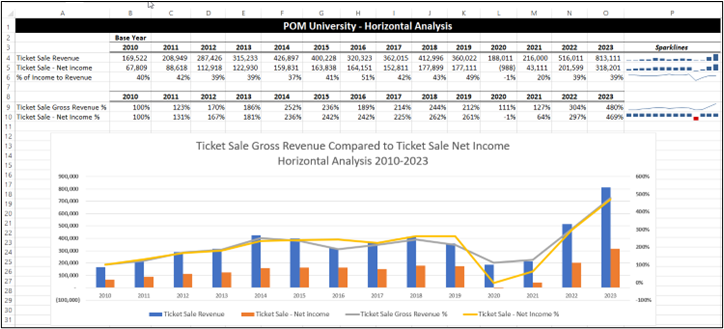
Look at 2010 and compare it to 2011. In 2011, the ticket sales gross revenue was 23% higher than 2010’s ticket sales gross revenue. In 2012, the ticket sales gross revenue was 70% higher than 2010. Note we always compare all ticket sales gross revenue for every year back to the 2010 base year.
The same is true for ticket sales net income. The year 2010 is the base year and is considered 100%. In 2011, the net income increased by 31% above the base year (2010). And in 2012, the net income increased by 67% over the base year (2010). Now the question might be, What is the purpose? The purpose is to help the audience determine historical patterns and determine the company’s potential growth. The combo chart shows that net income usually tracks at the same increased level as gross revenue increases; however, COVID-19 really disrupted this trend. Starting in 2022, it appears that gross revenue and net income were once more increasing together. This is good—it means the net income is currently trending with gross income. Essentially, expenses remain on track.
If you wish to explore combo charts, please review the Excel file associated with Chapter 3. Let’s turn to word clouds, a very easy visual with lots of uses.
What Is a Word Cloud?
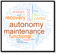
Word clouds are just visual representations of text in graphic form where the size of each word is relevant to importance or frequency. Essentially, the more often the word is used, the larger the text.

These keywords are evident in the pig image. This example was created on WordArt.com using the first 100 words in a story. I’m sure you can identify the story! Notice that even the shape tells you a little about the content.
Word clouds can be created in a multitude of ways, but one of the easiest to use is Word Art—Word Cloud Creator. This app is free to use but will add a cost to download high-quality images, though a standard download is free. This app even allows you to upload an image for the design. For example, a pig image was uploaded, and Word Art used this shape for the word cloud.
Word Art—Word Cloud Creator. Location: www.wordart.com
Remember, the pig example word cloud was generated from the first 100 words. There are several word cloud generators that work online without downloading any software. Most of them prompt you to copy or type text to generate the word cloud. And most, by default, start you with using the first 100 words. So how are word clouds used with large datasets?
Disruptor Intelligence Center: Global Data Uses Word Clouds
Some companies like Disruptor Intelligence Center: Global Data are using a Word Cloud to track what the top influencers in a field are talking about (and it is all live). The contributor indicates the topic based on a hashtag (e.g., #Infographic). In Exhibit 3.6 for BigData influencers, you can drill down into the resources and comments by selecting an influencer or start with the cloud and choose the topic of interest. Not everyone who reads this textbook will have access to Global Data, but if you do, read more about the features that follow.
Remember, the more a topic is discussed, the larger the word generated in the word cloud. In Global Data, choose Databases, and then under the Influencer Database, choose BigData. The illustration changes, since influencers use Reddit and Tweets to contribute, but you get a sense of what the influencers are talking about.
Exhibit 3.6—BigData Influencer Network With Word Clouds
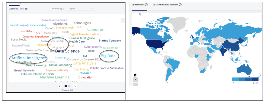
The word cloud is clickable, meaning if you select “Infographics,” it drills into the information to share the top contributors. The map shows the location and number of contributions. The database also lists the top contributors organized by the highest score. Twitter contributors are scored using (1) average engagements received on content shared, (2) number of followers, and (3) number of times other influencers have referred to them in their shared content. If you click on a contributor’s name, you will see the tweet content. One of our favorite contributors uses a lot of infographics to discuss big data, and once you find someone’s work you like, you can follow them.
Just a note: Global Data contains company information including a list of peers, SWOT analysis, PESTLE analysis by country, and many others. We will dive deeper into these basic tools and how to present key information visually in a later section.
Because a word cloud can identify trends and patterns, it is often used for qualitative research in an informal way. Most word cloud apps filter out common words, which means the visual shows patterns of frequency.
Keep in mind that most word cloud creators suggest the first 100 words of a story (but not all word cloud apps set a limit). For the word cloud demonstration, please use the following key information taken from a survey about leadership. Word Art is a little different. One way it functions is to allow the user to set up the frequency of words. Let’s look at a scenario to see how this might work.
Scenario: Survey Participants Ranked Leadership Characteristics
In this survey, participants indicated the following strengths for leaders. There were 30 participants. This means that all participants chose “Good communicator” as one of their top 10 leadership characteristics. In a word cloud, you would expect the phrase “Good communicator” to use the largest font. As you review the rest of the list, note the number beside it indicates how many participants indicated that strength as one of their top 10 leadership characteristics.
Table 3.1: Survey Participant Responses
|
Good communicator |
30 |
Empower others |
22 |
|
Fair |
22 |
Supportive |
22 |
|
Accountable |
18 |
Problem-solver |
17 |
|
Integrity |
16 |
Honesty |
15 |
|
Open-minded |
14 |
Creative |
12 |
Step-by-Step Approach to Create a Word Cloud Using Word Art
Note: Screenshots of WordArt.com © WordArt.com, https://wordart.com. Used with attribution for instructional and illustrative purposes. Annotations added by the author.
- Type www.wordart.com in your browser and sign up.
- Select the Create Now button (or the Create button if available). Notice that the pop-up menu has five sections: (1) words, (2) shapes, (3) fonts, (4) layout, and (5) style. In the words section, type the top 10 characteristics as shown in Figure 3.26.
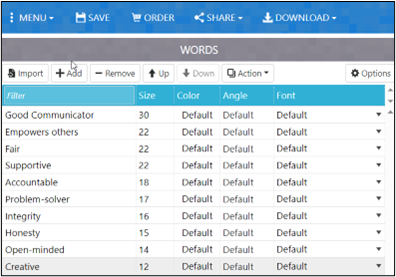
Figure 3.26—Setting up Survey Data in Word Art This is one of the easiest ways to work with survey data. If you wish to make a word cloud from a document, use the “import” command.
- Choose Shapes and for now, choose a square.
- Choose Fonts and choose League Gothic.
- Choose Layout and choose Horizontal/Vertical crossing.
- Choose Style to see what is there, but don’t change anything (you can always go back and change it later).
- Now to see your word cloud, choose Visualize. Each time you make a change, you need to use this button to see the changes.
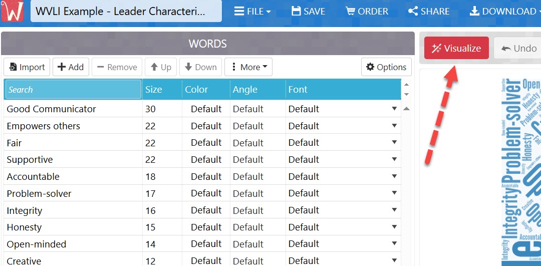
Figure 3.27 –Key Button to See Changes in Word Cloud - Choose Save in the blue menu bar.
Your image should look something like the illustration in Figure 3.28. To change any aspect and to see the changes, you will need to use the Visualize button each time you make a change to see the impact. Notice that if you hover the mouse over the words, they are animated.
Figure 3.28—Simple Word Cloud

Let’s look at some examples of other word cloud apps.
Add Pro Word Cloud to Microsoft Word
Perhaps more interesting is the add-in availability of Pro Word Cloud into Microsoft Word. Pro Word Cloud will generate a cloud based on a word count you set in Pro Cloud along with the act of highlighting the text. This feature is a great way to introduce a presentation based on a written document (like a strategic plan, business plan, or marketing plan).
Exhibit 3.7 depicts a sample word cloud created in Microsoft Word using the add-in, Pro Word Cloud. Only part of Chapter 2 was selected to create this word cloud, but we think it captured the main points pretty well!
Exhibit 3.7—Pro Word Cloud Capturing Part of Chapter 2
This cloud was created using the default settings in Pro Word Cloud.
Font—TANK
Colors—Default
Layout—Preserve Case
Case—Intelligent Case
Max Words:—5,000
Size (px):—600 × 372
Remove common words? Checked
Pro Word Cloud is just one of many add-ins that you can use to bring impact to your presentation or your narrative. Here are the directions for adding Pro Word Cloud to Microsoft Word (for a PC). Pro Word Cloud is a free app created by Orpheus Technology, and sponsored by Microsoft.
Step-by-Step Directions to Install Pro Word Cloud Add-In
Note: Screenshots of Word © Microsoft Corporation. Used with attribution for instructional and illustrative purposes.
- In Microsoft Word, on the ribbon, choose the Insert tab and Get Add-ins.
- Do a search for the term cloud and look for Pro Word Cloud as shown in Figure 3.29.
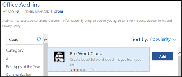
Figure 3.29—Office Add-Ins - Select Add and then Continue.
- Make sure to explore the many Office add-ins available. Many of them are free! Currently, there are more than 350 apps available just for Microsoft Word.
![]() Now that you have the Pro Word Cloud add-in, it is time to try it. (Don’t be surprised if you have to add it to Microsoft Word each time you want to use it!)
Now that you have the Pro Word Cloud add-in, it is time to try it. (Don’t be surprised if you have to add it to Microsoft Word each time you want to use it!)
- Open a Word document of your choice. Note how many words are in your document (lower left-hand area of your screen). The example used for demonstration is a draft of another chapter with 28,216 words.
- In Microsoft Word, on the ribbon, choose Insert.
- Next, choose My Add-ins and look for Pro Word Cloud.
- Choose the Pro Word Cloud and then click Add. It should add a Pro Word Cloud box on the right side of the document (see Figure 3.30).
Figure 3.30—Pro Cloud Instructions - Highlight part of or the entire document (do this with Control A on a PC).
- For now, just change the Max Words to 5,000 and keep all other default settings.
- Click Create Word Cloud and wait for Pro Word Cloud to generate the image (example shown in Figure 3.31).
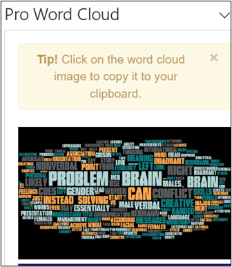
Figure 3.31—Word Cloud Example - Right-click the image to save as a picture.
- Try changing a few things and regenerate the word cloud to see the changes. Save any images you like.
There are tons of add-ins for Microsoft Word, but this is a very popular feature that is easy to use. But there are many ways to increase the interest level. For example, inserting the newly created word cloud into an image of the morning news makes a bold and more dynamic image than just the word cloud image alone.
Word Clouds Are Great as an Interesting Starting Point
Word clouds are great tools for specific situations. For example, a word cloud image is used in Exhibit 3.8 in conjunction with another app, essentially combining the word cloud image within the context of a newspaper.
Exhibit 3.8—A Fun Way to Use Your Word Cloud

The images were created using Pro Word Cloud. Just the Word Cloud image could have been used on a PowerPoint slide or within this document; however, the word cloud image was uploaded to PhotoFunia-Morning News to generate the image that combines it with a newspaper setting (date, newspaper title, and section) for a compelling way to start any conference session where you are the speaker! And what if you handed out coffee mugs for your session?
How Word Clouds Can Be Used for Surveys
Customer and Employee Surveys: Word clouds quickly indicate opportunities for improvement. Most survey tools provide a way to export data in several ways (text, Excel, PDF, CSV). That data can then be used in a word cloud generator. For example, the word cloud in Figure 3.32 is from a field on an exit survey. Administrators of the survey thought that “low wages” would be the key reason employees left, but based on the keywords and their size (displayed in Figure 3.32), the top three issues are (1) unfair treatment, (2) schedule, and (3) errors on paycheck. Most survey tools have an analytics section to summarize question answers; however, none of them has a tool to summarize written comments.
Figure 3.32—Employee Survey Word Cloud
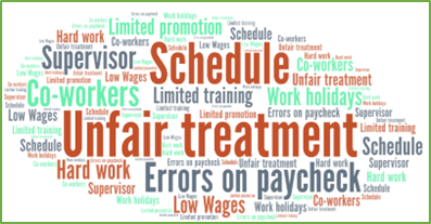
Just as a note—research shows that exit interviews should be conducted face-to-face (Glass Door for Employers, 2017). For example, in the previous situation, a face-to-face exit interview might shed some light on what is meant by “unfair treatment.”
Customer surveys are another area where you can gain insight into customer “pain” points, which provide insight into opportunities to improve and connect with your customers. In Figure 3.33, notice that a few phrases have been circled: slow, frustrating, and difficult. Although these words are represented by smaller text, it demonstrates that some customers did not have a positive experience.
Figure 3.33—Customer Survey Word Cloud

As you create word clouds, here are a few points:
- First, avoid simply dumping text into a word cloud generator. Take time to review what you are sending (this is called optimizing the data) to gain accurate insights. Consider what is relevant and important.
- Second, always consider if another visualization method will work better. For example, survey tools often have charts and graphs available for straightforward questions that provide limited ways to answer the question. More complex data might be better represented in a dashboard where they are interactive instead of static.
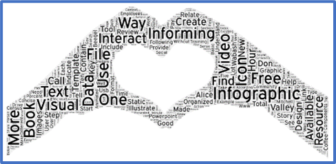
- Third, always consider how a shape might emphasize the message. For example, does the shape resonate with the data, or does it cause confusion? Many cloud apps will allow you to upload an image that can be used as the shape. Would a different shape (like Figure 3.34) add context and improve interpretation?
Figure 3.34—Shape of Infographic Designs
- Fourth, consider ways to customize or add interactivity if it enhances the audience’s insight. For example, you may notice that when your mouse hovers over a specific word, it pops up. You can record this activity with video editing software as well as add narration.
Please feel free to try some of the stand-alone word cloud apps.
WordClouds works with typed or pasted text, uploaded Office documents (even PowerPoints), PDFs, or text data. It also has a “wizard” for step-by-step help. Location: www.wordclouds.com
WordItOut has limited shapes and fonts, but it is very intuitive and easy to use. You can use text or even pull in words from a table or spreadsheet. Location: worditout.com/word-cloud/create
Interact With Your Audience Using Word Clouds
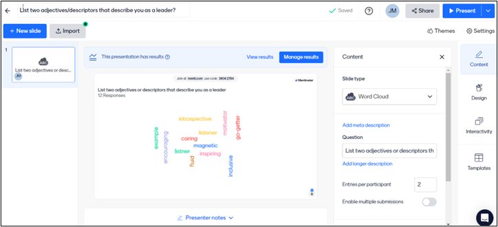
There are several products that allow you to use word clouds to interact with your audience—Here’s an example scenario: You’ve been asked to speak at a leadership conference, and you want to start the presentation with some audience interaction. Using an app like Mentimeter (www.mentimeter.com), you set up your slide with the prompt “List two adjectives/descriptors that describe you as a leader.” Your slide has a code at the top, and your audience uses their smartphones to connect to the presentation (www.menti.com) and type in the code (the code in this example is 3804 2784). The example shown in Figure 3.35 shows the setup along with a first attempt to test the interaction using my phone.
Figure 3.35—Using Mentimeter at a Conference for Interaction
Now it’s time to set one up for your next presentation! The free plan includes unlimited audience, unlimited presentations, up to 2 question slides, and up to 5 quiz slides.
The higher the frequency of a word, like any Word Cloud, the larger the word will be. A free version is available if your only plan is to use it for inspiration, but the price for the basic plan is under $11.99/month billed annually.
Interact With Your Team Using an Add-In to Microsoft Teams
Creating an interactive word cloud in Microsoft Teams is easy, and there are several ways to create it. The following demonstration is from one of my active teams. You should be able to follow along.
Step-by-Step Directions to Install a Word Cloud in Microsoft Teams (Poll)
Note: Screenshots of Microsoft Teams interface © Microsoft Corporation, used with attribution for instructional and illustrative purposes. Annotations added by the author.
- Open a team space of your choice. Within the team space, you will see a + at the end of the menu (see Figure 3.36).
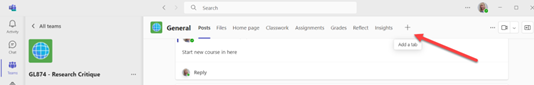
Figure 3.36—Add-In to Teams - When you click on the +, you should see a search bar that says Search for apps. If you don’t see the Poll app after typing Poll in the search bar, click the box that says Get more apps. You may see apps like Poll Everywhere, but you should look for the Poll app created by Microsoft.
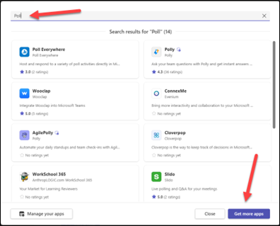
Figure 3.37—Adding Poll Everywhere to Teams - Once you click on Get more apps, Teams will open a categorized set of apps. Microsoft products have hundreds of apps available. Choose Popular on Teams and look for Polls. Figure 3.38 shows some of the more popular apps on Teams—another good one is Forms.
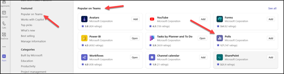
Figure 3.38—Apps Popular on Teams (Partial List) - Click Add and it will be added as a tab to your Team space. Once you add it, you will have the option to add to a team, add to a chat, or add to a meeting, as illustrated in Figure 3.39.
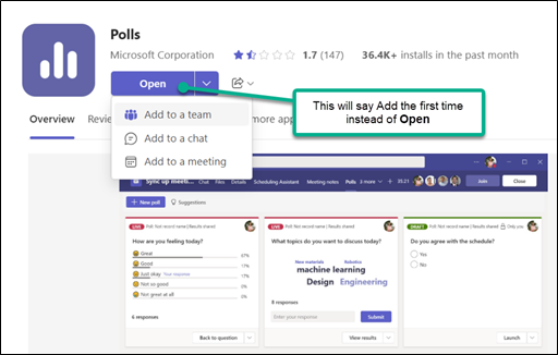
Figure 3.39—Choice of Where Polls Will Be Added - In Figure 3.39, the Polls app was added to a meeting, and then New Poll was selected. The pop-up provides choices available as of January 2024. Microsoft is continuing to update and add new features, so it is possible to see additional engagement activities. As seen in Figure 3.40, you can boost engagement with a word cloud, but other options are available.
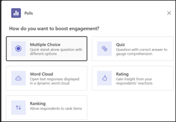
Figure 3.40—What Can You Do in Polls? - One of the things I like about this is the ability to Save as draft instead of Launch now. As the team members enter the meeting space, you can decide to launch when it is appropriate. If you launch the poll before the meeting starts, the team members will see the question that starts the process. It might be better to save it as a draft, as illustrated in Figure 3.41.
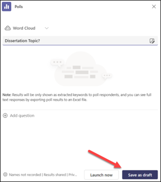
Figure 3.41—Setting Up Poll Question - If you set up the word cloud question before the meeting, the team members will see something like Figure 3.42 when they enter the team space (of course, with your question instead of mine).
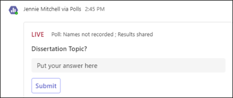
Figure 3.42—What Team Members See If Launched Before Meeting Starts
This is a great way to engage your audience without taking a lot of time. The following YouTube video shows how it was used with a live audience!
 Modern Work Superheroes. (2022, Nov 9). How to Use Word Cloud in Polls for Microsoft Teams. [Video]. YouTube.
Other Ways to Use a Word Cloud
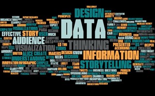
Figure 3.43—Word Cloud Showing a Research Study
The uses shown in Figure 3.43 for word clouds range from a simple visual of a text document to a more intentional use of looking at survey comments, but there are many other uses for word clouds.
In a recent study, word clouds were used as “text mining” of electronic health records. Essentially, “meaningful words were extracted . . . to perform pattern matching, followed by text mining and word cloud. . . . By combining these techniques, physiotherapy treatments could be characterized by a list of constructed keywords, and the residents’ health characteristics were built. Feeding defects or health outlier groups could be detected” (Delespierre et al., 2017, p. 1). If you look at the original article, this was much easier to understand than the text!
Most statistical software packages provide a way to create word clouds, but the apps shown in this chapter can help you with many word cloud projects!
3.2 Self-Assessment Recognizing Insights
Learning Objective #1—Determine insights
You have net income data for 10 years.
3.2 Exercise 1: Create Horizontal Stacked Bar Charts and a Word Cloud to Provide Insight
Learning Objective #1—Determine insights
Part 1
You work at a retail warehouse called “Just Stuff.” Over the past month your team has collected feedback from customers regarding their shopping experiences. The feedback covers various aspects and is summarized in Table 3.2.
Table 3.2: Summarized Feedback From Customers and Corresponding Chart
|
Category |
Excellent |
Good |
OK |
Poor |
|---|---|---|---|---|
|
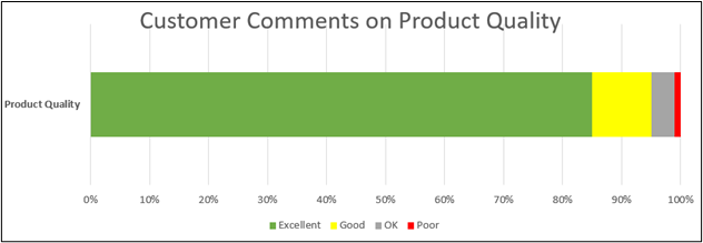
Product quality |
85% |
10% |
4% |
1% |
|
Product price |
75% |
5% |
19% |
1% |
|
Staff interaction |
50% |
10% |
15% |
25% |
|
Store environment |
60% |
11% |
10% |
19% |
|
Overall satisfaction |
70% |
5% |
9% |
16% |
The team chose the colors green for Excellent, yellow for Good, gray for OK, and red for Poor. The team envisions something like Figure 3.44 for each category.
Figure 3.44—Horizontal Stacked Bar Chart for Product Quality
Part 1 Assignment
- Create a horizontal stacked bar chart for each of the five components of the feedback summary (Table 3.2). The first one is completed for you.
- What insights can you share?
- What potential strategies would you recommend?
Caution—all charts should start at 0% on the x-axis!
Part 2
Besides summarizing the survey, your team members captured what customers said when asked to share their first impression from their shopping experience. Your team recorded the first thing said by the customer during the survey.
Table 3.3: First Impression
|
Great prices (50 customers) |
Staff disinterest (21 customers) |
|
Quality products (50 customers) |
Staff on phone (20 customers) |
|
Best prices (30 customers) |
Ignored (20 customers) |
|
Rude staff (22 customers) |
Dirty (18 customers) |
|
Missing cashier (18 customers) |
Windows need cleaned (16 customers) |
|
Bathroom needs cleaned (15 customers) |
Odd smell (14 customers) |
Part 2 Assignment
- Create a word cloud for the first impression (Table 3.3).
- Develop a short report highlighting your findings and include the five charts from part 1 and the word cloud from part 2.
- What insights can you share, and what strategies would you recommend?
Post the assignments per instructor directions. Your instructor may ask you to post the assignments to a discussion board, present your charts and word cloud and discuss your findings in class, share and present in a Teams meeting, or another option.
3.3 Benchmarking, Decision-Making, and Strategic Analysis Tools
Data visualizations must communicate answers and provide business outcomes. If the data feeding an analytics dashboard is not trusted, the results are meaningless. If the visualizations do not answer important business questions, the visualizations are not actionable.
—Katie Horvath, CoreSignal
Today, data-driven decision-making is foundational for global business. As the quote from Katie Horvath suggests, managers and researchers must present data that is accurate and unbiased. At any point, if trust is lost, the results are meaningless. The integrity of decisions rests on the ethical handling and presentation of data. Storytellers need to ensure that biases (international or otherwise) do not distort the information conveyed.
Benchmarking is the process of comparing performance metrics (like key performance indicators [KPIs]) against established standards. Organizations rely on benchmarking to assess progress, identify areas that need improvement, and gauge the effectiveness of strategies. Metrics can help measure targets related to process, strategy, and performance. Yet the way data are presented can profoundly influence perceptions and decisions. This section explores the intersection of benchmarking and ethical practices in data presentation. For this chapter’s purpose, consider four types of benchmarking: (1) performance benchmarking, (2) practice benchmarking, (3) internal benchmarking, and (4) external benchmarking. Every industry should use benchmarking to help understand and transfer “best practices” from other organizations and improve organizational performance.
Internal and External Benchmarking
Internal benchmarking involves comparing different units, departments, or processes within the same organization. For example, a retail company with multiple store locations can survey customer satisfaction. Next, the company identifies the store location with the highest customer satisfaction. The organization would analyze this location’s processes, training methods, and customer engagement strategies and share the insights gained company-wide.
External benchmarking involves comparing an organization’s processes, performance, and/or practices with those of another organization, typically in the same industry. There is a plethora of tools that can be used to benchmark your organization to your competitor and your industry. For example, to understand the competitive environment of an industry, use Porter’s Five Forces and Porter’s Generic Strategies (both tools were developed by Michael Porter, an economist at Harvard). Let’s look at these from an external benchmarking point of view.
Benchmarking Tool 1: Porter’s Five Forces
One of the best benchmarking tools to understand industry competitiveness is Porter’s Five Forces because industry leaders recognize the components. For example, MarketLine Advantage is a world-leading provider of industry profiles that include Porter’s Five Forces. MarketLine Advantage showcases over 30,000 companies, over 3,500 industry profiles, and over 110 country profiles (MarketLine Advantage Brochure, 2023). MarketLine uses Porter’s Five Forces analysis framework “to evaluate the competitive pressures on ‘players,’ rival companies in a particular market” (MarketLine Advantage Brochure, 2023). Industry profiles include five-year forecasts, practical application of Porter’s Five Forces analysis, and company financial metrics. Most college libraries have access to the MarketLine Advantage tool. Let’s start by looking at an industry profile.
Industry Profile—Global Cloud Computing
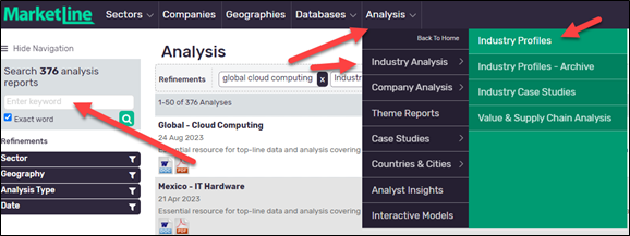
The August 2023 Global Cloud Computing Industry profile is 44 pages of relevant information on the state of global cloud computing. Based on the table of contents, the industry profile includes an executive summary, market overview, market data, market segmentation, market outlook, (Porter’s) Five Forces analysis, competitive landscape, company profiles (this includes financials in most cases), and macroeconomic indicators. Figure 3.45 shows the journey to finding the Global Computing Industry profile. From the main menu, choose Analysis, Industry Analysis, and then Industry Profiles. Or you can use the search feature to find it. Industry profiles are updated often.
Figure 3.45—Industry Profiles in MarketLine
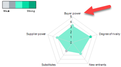
If you open the global cloud computing profile, the five forces are buyer power, degree of rivalry, new entrants, substitutes, and supplier power. But what I really like is the graph, “Drivers of Buyer Power.” MarketLine dives into each of the five categories. For example, in Exhibit 3.9, looking at buyer power, the following factors are measured: backward integration, buyer independence, buyer size, financial muscle, low-cost switching, oligopsony threat, price sensitivity, product dispensability, tendency to switch, and undifferentiated product. A relevant chart is supplied for each of the five forces to show the drivers.
Want to learn more about Porter’s Five Forces?
Expert Program Management (EPM). (2021, Jun 14). Porter’s Five Forces explained with example [Video]. YouTube.
De Bruin, L. (2016, Aug 3). Porter’s Five Forces. Business-to-you. https://www.business-to-you.com/porters-five-forces/
Exhibit 3.9—Five Forces and Drill Down Into Drivers for Buyer Power
|
Porter’s Five Forces driving competition global cloud computing industry, 2022 |
Porter’s Five Forces drivers of buyer power global cloud computing industry, 2022 |
|---|---|
 |
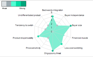 |
These are radar charts (which is a chart you can prepare in Excel). Radar charts are great for visualizing how entities perform across multiple dimensions and to help identify areas of focus for improvement or further development.
Another aspect of an industry profile is the competitive landscape. This section identifies the leading players. The 2023 global cloud computing industry profile identified these top players in the cloud computing industry.
- Amazon Web Services (AWS), a subsidiary of Amazon.com
- Microsoft (Azure platform)
- Google Cloud, a subsidiary of Alphabet Inc.
- IBM Cloud, of International Business Machines Corporation
- Alibaba Cloud, a subsidiary of Alibaba Group (and one of the fastest group cloud computing players located in China)
Because this is a textbook on leveraging data visualization, it’s important to understand how to build a radar chart using the global cloud computing industry as an example and an estimate of where the two players (AWS and Alibaba) are located. The numbers assigned to AWS and Alibaba in the “Step-by-Step Approach to Build a Radar Chart in Excel” are estimated and are for learning to build a radar chart.
Step-by-Step Approach to Build a Radar Chart in Excel
- Open the Excel file “3.3 Radar Chart” for this chapter.
- Find the tab 3.3 Radar Chart.
- The data for this how-to section are in Figure 3.46.
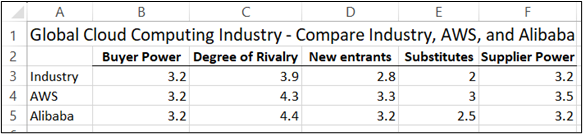
Figure 3.46—Data for Radar Chart - Highlight A2:F5.
- Choose Insert on the main menu.
- Select Recommended Charts.
- In the pop-up, select the tab All Charts.
- Scroll down to Radar.
- As shown in Figure 3.47, choose the first radar chart, or if you like the data points, choose the second one. Do not choose the fill one because this is a comparison.
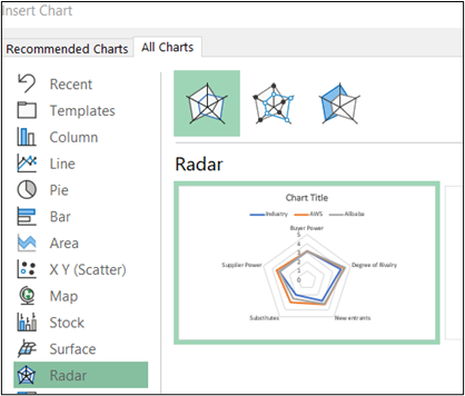
Figure 3.47—Choose First Radar Chart
Source: Screenshot of Excel Interface © Microsoft Corporation
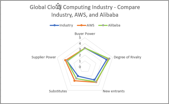
The final comparison shown in Figure 3.48 uses the second radar chart showing the datapoints.
Figure 3.48—Radar Chart for Industry, AWS, and Alibaba
How to Interpret This Radar Chart
In this radar creation exercise, the estimate of Porter’s Five Forces for each company was created for data visualization purposes. Although the industry data from the global cloud computing industry profile is accurate, the company numbers were created solely for this how-to demonstration. To interpret the results, compare the polygons of the different entities. Entities with polygons that are closer to the outer edge perform well in those corresponding variables. Entities with polygons closer to the center indicate weakness in those areas. This radar chart represents two companies ranked in the top five. Our results for a struggling company or a new entrant would yield very different results. In Figure 3.48, AWS slightly outperformed Alibaba.
Strategies That Follow Porter’s Five Forces Analysis
According to Michael Porter (2008), in his article “The Five Competitive Forces That Shape Strategy,” there are strategies that can be used to reshape the five forces. The strategies outlined by Porter include
- neutralize supplier power,
- counter customer power,
- temper price wars,
- scare off new entrants, and
- limit the threat of substitutes.
Let’s look at them using the context of the cloud industry.
Table 3.4: Strategies to Reshape the Five Forces
|
Neutralize supplier power |
Standardize specifications for parts so more vendors can provide them. This is a great strategy for the cloud industry since data centers rely on servers and processors, and normally have a well-established network of suppliers. |
|---|---|
|
Counter customer power |
Expand services so it’s harder for customers to leave. This is one strategy that Amazon Web Services has done successfully and now Alibaba is practicing as well. |
|
Temper price wars |
Invest heavily in products that differ significantly from competitors. In the cloud storage industry, all competitors rely on specific computer parts, and since many of these parts come from outside the United States, Amazon Web Services has a difficult challenge. Consider collaboration—Microsoft and Oracle are usually competitors, but they are working together in the cloud industry realm. |
|
Scare off new entrants |
Elevate the fixed cost of competing by investing in R&D and artificial intelligence. Or apply for patents that support cloud service innovations. |
|
Limit the threat of substitutes |
Offer better value through wider product accessibility. |
How Can Bias Creep Into Porter’s Five Forces Analysis?
Bias can creep into the content development of Porter’s Five Forces analysis in several ways. Bias creeps in when analysis becomes too narrow, you make untested assumptions, or your analysis is focusing on the wrong industry (this happens because companies often straddle more than one industry). Again, Michael Porter shared additional situations that can reduce profits:
Bias #1—Savvy customers
- You think you know your customers, and assume brand loyalty, but according to the State of Cloud 2023, 65% of organizations use a multicloud environment (Pluralsight, 2023). “Savvy customers can force down prices by playing you and your rivals against each other” (Porter, 2008, p. 24). An organization that uses a multicloud strategy will use two or more cloud providers to take advantage of the capabilities that best suit their purpose as well as prevent vendor lock-in.
Bias #2—Powerful suppliers
- “Powerful suppliers may constrain your profits if they charge higher prices” (Porter, 2008, p. 24).
Bias #3—Entrants
- “Aspiring entrants, armed with new capacity and hungry for market share, can ratchet up the investment required for you to stay in the game” (Porter, 2008, p. 24).
Bias #4—Substitutes
- In the case of cloud computing, the types of services are identical but when you perform the analysis, you may assume brand loyalty that is not there.
An Introduction to Porter’s Generic Strategies
The term generic strategies was first introduced by Michael Porter and upon review, is reminiscent of Management 101. This model introduces strategies to gain a competitive advantage. It includes cost leadership, differentiation, and focus. To apply a cost leadership strategy, your organization would:
- increase profits by reducing costs (still charging industry-average prices).
- increase market share by charging lower prices (still making a reasonable profit).
Cost leadership is not for every organization. To apply this strategy, you need technology to bring costs down, efficient logistics, and a way to sustain the lower costs.
To be successful at differentiation strategy an organization needs:
- good research, development, and innovation,
- to be able to deliver high-quality products or services, and
- a marketing team that understands how to market differential products and services.
The third strategy focus is used in conjunction with cost or differentiation; Porter calls this Cost Focus and Differentiation Focus, and you should not try to do both. The process to use this model includes these steps:
- Conduct a SWOT for each potential strategy. What strengths, weaknesses, opportunities, and threats would result in the strategy chosen?
- Use Porter’s Five Forces and PESTLE to understand the industry and the environment.
- Compare SWOT and Porter’s Five Forces and choose one generic strategy that gives you the best set of options.
For more information about Porter’s Generic Strategies and example organizations that have applied the model, check out the following link.
De Bruin, L. (2021, Apr 14). Porter’s Generic Strategies: Differentiation, cost leadership and focus. Strategic Planning—B2U Business-to-you. https://www.business-to-you.com/porter-generic-strategies-differentiation-cost-leadership-focus/
Benchmarking Tool 2: Comparative SWOT
Once you analyze your industry using Porter’s Five Forces, the next step is to review SWOT analysis of the organization (or players) in this industry. In this same MarketLine Advantage database, each of the players shows a company summary, key statistics, research reports, deals, and a SWOT analysis. As you may recall, a SWOT will show strengths, weaknesses, opportunities, and threats. Strengths and weaknesses are considered internal, and opportunities and threats are considered external.
Once a company conducts a SWOT (either for their own organization or compared to a competitor), the next step is to develop strategies and action plans based on the insights gained from the analysis. These include the following:
- Capitalize on strengths: Leverage a company’s strength to gain a competitive advantage.
- Address weaknesses: Work to improve identified weaknesses and develop plans to enhance capabilities, skills, processes, or resources pertaining to areas of weakness.
- Exploit opportunities: Capitalize on external opportunities that align with the company’s strengths.
- Mitigate threats: Develop strategies to minimize the impact of external threats on the business by creating contingency plans, diversifying offerings, or strengthening relationships.
Remember a SWOT analysis is only valuable if it leads to meaningful action.
Figure 3.49 compares the leading player, Amazon, to the organization ranked fifth, Alibaba Cloud. The SWOTs consider the following categories: operational, financial, strategic, industry, political environment, economic situation, sociocultural environment, and technological environment.
Figure 3.49—An Example Comparison SWOT Analysis
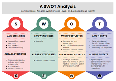
One of the greatest weaknesses for growth is for an organization to be in the position of declining cash, especially if capital (interest costs for borrowing) is more difficult to raise. Let’s look at another benchmarking tool that adds another layer of understanding to the situation, especially if you hope to expand your company into a new country.
A PEST/PESTLE adds another layer of understanding to your organization’s situation. It is a simple and effective tool used to identify the key external forces at a macro environment level. A SWOT is not complete unless you conduct a PEST or PESTLE.
Benchmarking Tool 3: PESTLE (Also a Strategic Analysis Tool)
A strategic analysis tool should be used anytime your company is considering expansion into a new geographic area. PESTLE analysis incorporates: P = political (or sometimes referred to as politics), E = economical, S = social, T = technological, L = legal, and E = environmental. MarketLine uses PESTLE and PEST as part of the country analysis framework. So for companies considering expanding their market, this is a critical tool.
For example, one of MarketLine’s PESTLE analyses is for the country Japan. The insight document (Japan In-Depth PESTLE insights) was published in January 2020 and is 96 pages long! But you can apply this analysis technique in a much smaller way. It is a pretty good model for expanding a market anywhere. Here are some considerations when conducting this analysis.
- Political: What is the current taxation policy and what changes are they considering? What is the political outlook?
- What trading policies impact your business?
- What are the specific regulations that you need to follow, and have they changed?
- Is there current legislation that might impact your business?
- Economical: What is the overall economic situation? Is there a growing strength in consumer spending?
- Does globalization affect your market share?
- Is the economy stable? Growing? Declining?
- Do you understand the taxes that are applicable to your product or service?
- Is the government fighting loan deficits?
- Social: What lifestyle or trends are there to consider? What is the demographic of the consumer? Are there attitudes or opinions that should be considered?
- Who is your target market?
- Is the population growing and do they have a need for your product or service?
- Technological: Do they have relevant technology and innovations?
- What technology is critical to support your operations and/or do you need vendor support? And if you need vendor support, are they in-country?
- Does their technology infrastructure support your needs?
- Does the country have weak intellectual property laws?
- Legal: Is there legislation in areas that would impact the company? For example, employment, tariffs, health, or safety. Are there labeling laws required?
- Is the country transparent or is there evidence of corruption?
- Are there hidden tariffs?
- Does your organization understand the country’s taxation structure (e.g., value-added tax [VAT] is often a surprise to companies when they expand into Europe).
- Environmental: Would a company product contribute to pollution? Are there recycling laws that would impact manufacturing the product or consumer use of the product?
- What international treaties are signed in relation to air pollution, ozone layer damage, or disposal of hazardous waste?
Combine your analysis with a great graphic like the one illustrated in Exhibit 3.10, which helps visualize the insight analysis. You can create a PESTLE analysis in PowerPoint or one of the infographic software packages.
To illustrate how a PESTLE might be used, assume that Amazon Web Services (AWS) is investigating expanding into Greece. This potential expansion should always include a review of the PESTLE landscape. MarketLine provides a country profile for Greece. The March 2023 country profile is 82 pages long, but this small graphic (Exhibit 3.10) captures the key points.
Exhibit 3.10—Comparison of a PESTLE for Greece
|
Created in PowerPoint |
Created in Venngage |
|---|---|
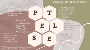 |
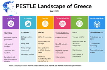 |
The type of background and layout is important. The Venngage example shows PESTLE all aligned, implying that each one carries the same weight; however, that is not true, and it will vary by industry.
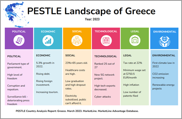
To leverage data visualization and tell the story, begin with a brief introduction that highlights the purpose and provides context to the audience. Share an example that demonstrates the importance of understanding external factors. Next, present a clear structure. Obviously, your audience can’t read all the fine print, so set up a section for each factor. Each section should include a brief overview, impacts on the organization, specific examples, and trends.
For example, Greece has just started a project to place a 5G network throughout the country. As a cloud computing company, they would want the 5G network in place, and hiring talent might be an issue because of the low graduation rate at the tertiary (college) level. Amazon Web Services would want to evaluate these factors based on their unique situation.
In Figure 3.50, notice the minimum wage of $750.50 EUR/month. Does that surprise you?
Figure 3.50—PESTLE Landscape of Greece in 2023
There are several variations for this strategic analysis tool, including PESTEL (just a different ordering), PEST (where companies do not consider legal and environment), and PESTELE or STEEPLE. The PESTELE or STEEPLE represents a variation that includes “ethical and industry specific factors.” For example, this area would include such components as fair trade, child labor, and corporate social responsibility (CSR).
Benchmarking Tool #4—Compare With an Association Database(s)
Most industry associations provide benchmarking data specific to their sector which allows you to compare your organization’s performance with industry norms. Examples include American Hotel & Lodging, National Retail Federation, Automotive Industry, Hospital Association, and National Collegiate Athletic Association (NCAA). There are hundreds more.
If your organization is required to report information, you can assume that the data collected is analyzed in some way. For example, the U.S. Department of Education sponsors the Equity in Athletics Data Analysis (EADA). The EADA is a report required by the U.S. Department of Education’s Office for Civil Rights under Title IX regulations. The EADA report provides information about the participation rates, financial support, and other aspects of intercollegiate athletic programs at higher education institutions.
U.S. Department of Education. (2023). Equity in Athletics Data Analysis. https://ope.ed.gov/athletics/#/
Bias in Reporting Data
The reporting of academic data, including average GPA for student athletes can vary widely from one institution to another. Although the data are collected as part of the NCAA Academic Progress Rate, it does not require a direct measure of average GPA; however, it does consider academic eligibility and retention of student athletes. Institutions that fail to meet these thresholds can face penalties and loss of scholarships. There is no requirement to post athlete GPA for public viewing, but many institutions want to be both accountable and transparent and post some type of infographic about team GPA or sport-wide GPA. Here’s the catch! Some institutions post GPA data when they are good and fail to post anything about student athlete GPAs when they are low.
In Exhibit 3.11, note how internal and external benchmarking might be used from an infographic perspective. Most colleges and universities track the GPAs of their athletes, and it’s fairly common practice for any college or university to track their athletes’ academic journeys (internal). However, some colleges have a spotty record of posting GPA information for public view (external).
Exhibit 3.11—To Post or Not to Post Average Student Athlete GPA
 |
 |
| Washington State University. (2022). WSU Athletics Spring 2021 Academic Highlights. Available: https://news.wsu.edu/athletics-spring2021-academic-highlights-infographic/ | Holy Cross Crusaders. (2019). Holy Cross News. Spring 2019 Holy Cross Athletics—Academic Highlights. Available: https://goholycross.com/news/2019/7/1/211806300.aspx |
Now the question is, Do you see the GPA of college athletes posted for your institution?
Benchmarking Tool #5—Balanced Scorecard
There are several types of performance metrics that should be considered for your organization. Organizations need performance indicators to measure performance and the organization’s ability to reach their goals.
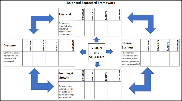
One of the first in this section is a Balanced Scorecard (BSC). This benchmarking tool was first introduced by David Norton and Robert Kaplan in the late 1990s. BSC is considered to be one of the first performance metric tools to take into account nonfinancial information. The BSC measures four main aspects: learning and growth, business processes, customers, and finance (or for a nonprofit, instead of customers, it can be donors).
Figure 3.51 visually depicts what it might look like at the very early stages (this illustration was created in Excel and is included in the Excel files for this chapter).
Figure 3.51—Early Rendition of Balanced Scorecard Framework
Since the late 1990s, the BSC has been used and modified by organizations. You will often see key performance indicators (KPIs) instead of measures and projects instead of initiatives. Instead of learning and growth, you might see organizational capacity. The framework for organizational capacity (financial, customer, internal processes, and the newer perspective) is often found in the form of a strategy map.
A strategy map is a visual depiction of cause-and-effect connections between strategic objectives. When used in conjunction with BSC, a strategy map is used to communicate how value is created by the organization. An example strategy map is shown in Exhibit 3.12. According to Kaplan & Norton (2001), “A strategy map enables an organization to describe and illustrate, in clear and general language, its objectives, initiatives, and targets; the measures used to assess its performance . . . and the linkages that are the foundation for strategic direction” (para. 14).
One of the easier industries to review is the airline industry. The cost of the flight is the same if the plane is full of passengers or if it carries only a few passengers, so it should be no surprise that standardizing planes for quick ground crew turnaround will increase customer satisfaction, since travelers hate delays for many reasons (connecting flights, losing quality time, etc.).
Exhibit 3.12—Sample Strategy Map Used With BSC
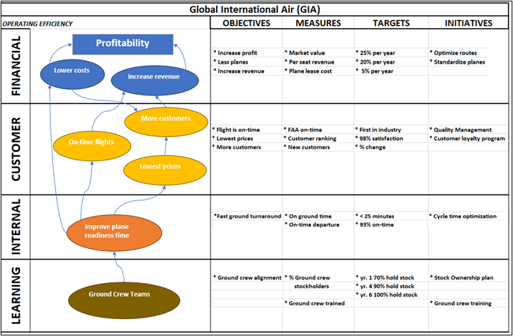
Although implementing a balanced scorecard framework can lead to substantial positive change, about 30% of BSC initiatives fail. The less-than-optimal outcomes can be caused by a lack of leadership and commitment (especially buy-in). This lack of leadership has several symptoms including unclear strategies, inadequate communication or mixed signals, incorrect metrics, or overemphasis on just the financial metrics. BSC has been around for over 30 years, and 70% of Fortune 1,000 companies have at least partially implemented a BSC (BSC Designer: Balanced Scorecard Fact Sheet, 2023). According to the “Management Tools & Trends,” the BSC tool is one of the top three most popular business tools (Bain & Company, 2023).
Incorporating a dashboard in conjunction with a BSC framework can bridge the gap between strategy and execution by providing real-time insights. It’s effective because it makes it easier for organizational stakeholders to monitor, analyze, and take action based on performance data. Let’s look at the illustration in Exhibit 3.13 to learn more.
Exhibit 3.13—Simple (Partial) Example Dashboard to Support BSC
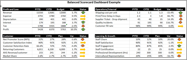
This example dashboard can support a BSC in several ways:
- centralized performance
- visual representation (the arrows) where stakeholders can see patterns and trends
- real-time monitoring, possible with built-in performance alerts
- customization (this is a very simple dashboard—many have lots more visuals)
- reinforced alignment between strategic objectives and the metrics being tracked (by organizing metrics along BSC)
- communication and decision support
- comparative analysis with historical data
To learn more about BSC, feel free to watch the following YouTube videos. The first provides the basics, and the second video is an interview with Professor Kaplan (one of the creators of the Balanced Scorecard).
Business School 101. (2022, Oct 31). Balanced Scorecard (with a step-by-step example) from a business professor [Video]. YouTube.
CPA Strategic Management Accounting. (2023). CPA R. Kaplan explains the Balanced Scorecard. knowledge equity [Video]. YouTube. https://www.youtube.com/watch?v=4xXwFwQmRIM [Embedding disabled for this video.]
Sector Scorecard by Global Data (Disruptor)
Global Data uses a scorecard approach “to predict tomorrow’s leading companies within each sector” using thematic, valuation, risk, and company screen (2023). The thematic screening ranks companies based on overall leadership by 10 themes most valued by their industry. The 10 themes are different depending on the sector. So for cloud computing services, you will see artificial intelligence, software-defined networks, internet of things, enterprise SaaS, cloud IaaS, hybrid cloud, edge computing, multicloud management, AI chips, and Metaverse. The legend indicates that green will impact earnings positively, yellow is neutral, and red will have a negative impact on earnings. The use of red, yellow, and green is symbolic in the United States, similar to a traffic light.
Exhibit 3.14—Thematic Scorecard of Cloud Service Sector (Partial)
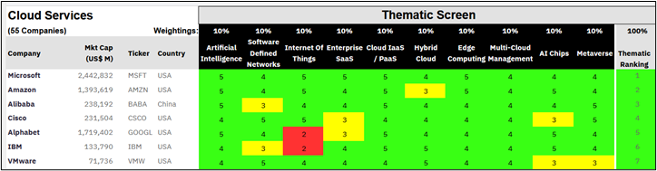
Although Exhibit 3.14 shows an overall positive impact on earnings, this is only a partial view of this scorecard. As you move down to companies ranked 25–65, expect to see a lot of red and yellow with very little green.
Personal Individual Strategy Map
The BSC can be translated into your own personal, individual strategy map. The example illustrated in the strategy mapping article shows a faculty strategy map from an academic perspective. The strategy map for an academic in higher education can guide personal development and define objectives in teaching, research, and service. Even more appealing is that the strategy map can help faculty members focus on strategies and should be created at the beginning of the academic year.
Novice educators should determine how setting one objective can contribute to the success of another. For example, successful research publication could enhance teaching effectiveness. The key performance indicators (KPIs) track progress toward each objective (like course evaluations, number of publications, grants, service committees, etc.).
The takeaway from this section is that strategy maps aligned with BSC perspectives provide a dynamic evaluation of your company with multiple views.
Adamson, K. (2019, Jan 23). Strategy mapping: An essential tool for new academic faculty. Faculty Focus. https://www.facultyfocus.com/articles/faculty-development/strategy-mapping-an-essential-tool-for-new-academic-faculty/
3.3 Self-Assessment Benchmarks
Learning Objective #4—Create and use benchmarking frameworks to provide context for problem, support decisions, and measure performance
3.3 Exercise 1: Analysis of Industry Profile, Leading Players, and SWOT
Learning Objective #2—Use benchmarking, decision-making, and strategic analysis tools
(This exercise assumes you have access to MarketLine in your university’s library.)
Create a professional report that has three main components: (1) information about the industry, (2) two-company comparison of SWOTs from top players from the industry, and (3) a discussion of Porter’s Five Forces.
Step 1: Start at MarketLine Advantage and find an industry profile.
Step 2: Go to the industry profile section, which lists the top players.
Step 3: Go to the company section in MarketLine and make sure that at least two of the companies from your industry profiles have SWOTs listed. If not, choose a different industry.
Step 4: From the industry profile, review Porter’s Five Forces. Discuss trends and challenges for the industry. Summarize the important aspects of the industry.
Step 5: Pick two of the top players (that have SWOTs) and do a comparative SWOT. Compare and contrast the two players. What challenges do they share? Why are these two companies outperforming other companies from the same industry? Which company is stronger externally (opportunities and threats)?
What should the report contain?
- A discussion of Porter’s Five Forces and the supporting factors. Feel free to capture the radar chart as a screen capture—just make sure to cite it.
- A discussion of the industry and the two players (that you chose)
- Summarize important information about the industry.
- An infographic comparing the SWOTs
- A discussion comparing the two companies
- Which company is stronger internally (strengths and weaknesses), and which company is stronger externally (opportunities and threats)?
- What components are similar?
- Did the industry profile analysis indicate similar internal or external factors to the SWOT analysis? Create an infographic comparing the SWOTs from the two companies.
- Create a radar chart comparing the two companies.
Other aspects required are as follows:
- well-organized professional template with headings
- no spelling errors, typos, or grammar issues
- appropriate APA citations
Hint: You may want to look for professional report templates. Microsoft has dozens of paper and report design layout templates.
Check with your instructor to see if they prefer a PowerPoint presentation instead of a professional report.
3.3 Exercise 2: Create a SWOT for Your Organization
Learning Objective #2—Use benchmarking, decision-making, and strategic analysis tools
Complete research on your organization, the history, the industry, trends, and so on. What is your industry? Who are your competitors?
Create a SWOT infographic for your organization. Include a discussion that outlines your thought process. Remember S and W are internal, and O and T are external.
3.3 Exercise 3: Conduct PESTLE Research
Learning Objective #2—Use benchmarking, decision-making, and strategic analysis tools
(This exercise assumes you have access to MarketLine in your university’s library.)
Step 1: Go to MarketLine and choose Country Profiles.
Step 2: From the country profile, create a PESTLE infographic.
Share the infographic and be prepared to discuss the company profile.
3.3 Exercise 4: Balanced Scorecard
Learning Objective #2—Use benchmarking, decision-making, and strategic analysis tools
Learning Objective #4—Create and use benchmarking frameworks to provide context for problems, support decisions, and measure performance
(This assumes that students have access to the ProQuest eBook Central database at their university.)
Step 1: Go to the ProQuest eBook Central database and find Management Accounting Case Book.
Step 2: Go to pages 71–78 within the case book and read “The Tri-Cities Community Bank: A Balanced Scorecard Case.”
Step 3: Complete the following components of the case (the page numbers and exhibit names are from the case).
- Question 1 (p. 73): Create a table that categorizes each of the measures in Exhibit A2 into one of the four BSC perspectives. Exhibit A2 is in the case “The Tri-Cities Community Bank: A Balanced Scorecard Case.”
- Question 2, modified (p. 73): Create a cause-and-effect chain using the one shown in Exhibit 3 as an example. Use the measures listed in Exhibit A2 or suggest other measures you feel are appropriate. Include an explanation.
- Question 3, modified (p. 75): Graph the key performance indicators on Exhibit B1 using the most appropriate graph type in a dashboard style. Discuss the implementation quality that may explain variation in performance among branches A–E. What implementation recommendations would you make to the ND managers considering the key performance indicators and your interaction with them?
Case Citation
Lawson, R. A. (Ed.). (2020). Management accounting case book: Cases from the IMA educational case journal. John Wiley & Sons, Incorporated. ProQuest eBook Central Database.
3.4 Visual Decision-Making Tools
Data visualization is the language of decision making. Good charts effectively convey information. Great charts enable, inform, and improve decision making.
—Dante Vitagliano, CoreSignal
Visual decision-making tools can illuminate pathways to effective choices. This section delves into several decision-making tools that have visual representations. Early in this section, fill out the interconnected bones of Ishikawa diagrams to drill into the core problem instead of just treating the symptoms. Next, learn to build the structured branches of decision trees to weigh a decision using probability theory. Learn to use the discerning lenses of Pareto analysis to concentrate resources to gain the most impact. This section even includes the House of Quality used for the streamlined precision of Six Sigma methodologies. This section provides practical guidance on how to wield these tools effectively, leveraging the visualization output to communicate effectively.
Decision-Making Tool 1: What Is an Ishikawa Diagram?
An Ishikawa diagram was invented several decades ago by Kaoru Ishikawa to help a team identify and arrange the causes of a problem. It is a brainstorming tool that can help a team organize, visualize, and communicate. Often teams use sticky notes to think of all the causes that contribute to a specific problem. You can still do that! Just start with five or six categories and build your fins. For example, assume that you have a coffeeholic in your family. Your categories might look something like Figure 3.52 created in Visio (i.e., people, procedure, materials, and equipment). Notice that Visio provides a fish frame as well as primary and secondary cause shapes.
Figure 3.52—Ishikawa Diagram: Determine Categories.
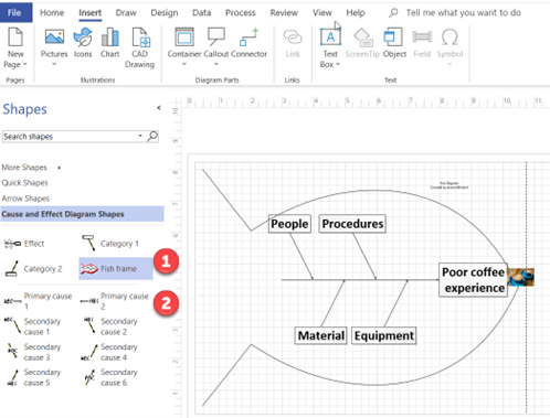
Next, have your team review each sticky note and arrange them into categories. Some example “causes” are shown in Table 3.5 for the problem “poor coffee experience” under the categories listed earlier.
Table 3.5: Brainstorming Example Causes
|
Procedure |
Material |
People |
Equipment |
|---|---|---|---|
|
Grounds in my coffee |
Don’t carry my sweetener |
Rude |
Cold coffee when I want hot |
As you start to build out the diagram (as shown in Figure 3.53), you will probably think of other causes that lead to a “poor coffee experience,” especially if you are a coffee drinker!
Figure 3.53—Partial Ishikawa Diagram
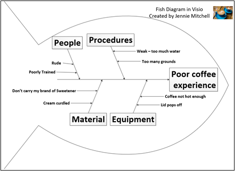
Categories can be customized based on the problem. If your organization is a manufacturer, you might see categories using the five Ms of manufacturing (manpower, machines, materials, methods, and measurements). If your organization provides services, expect the six Ps (people, processes, policies, procedures, places, and performance). But know that you can customize the categories to fit your situation.
The “problem” is situated toward the nose of the fish, and the causes (and subcauses) are pointed to the spine of the fish. Don’t be surprised if you need to change your problem statement. For example, we started with “bad coffee” as the problem statement, but then saw that an employee being rude didn’t really impact the taste of the coffee. Instead, it became clear that the real problem was a “bad coffee experience” related to visiting the local coffee shop.
Depending on the software or app that you use, the Ishikawa diagram could be called a root cause analysis or fishbone diagram. Exhibit 3.15 was created in Visio and shows the shapes and images that can be used. Note these are linked to primary causes, secondary causes, and so forth.
Exhibit 3.15—Sample Fish Diagram
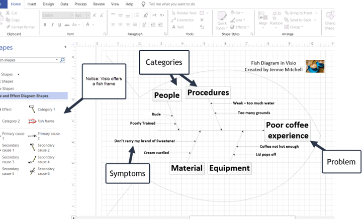
Did you know that brainstorming is one of the most creative ways to solve a problem? And doing it with a team provides some additional benefits. Brainstorming can
- reduce social inhibitions among group members,
- stimulate ideas that you might never consider,
- enlighten the impact of the problem across departments, and
- capitalize on multiple perspectives.
You don’t have to have a fancy fish diagram. You could even create a fish diagram in a Word document, but why create it yourself when there are templates and apps that will do it for you?
An Ishikawa diagram can be more dynamic if you use hyperlinks and the Zoom feature in PowerPoint, but there are dozens of videos on YouTube to enhance your storytelling. Watch Chad Littlefield’s video “How to Make a PowerPoint Presentation Interactive” to consider ways to interact with your audience like the two-minute Google activity, contribution-not-consumption, Wikipedia Game, bringing an object in physically, a translation technique, and optical illusions.
Littlefield, C. (2021). How to Make a PowerPoint Presentation Interactive. [Video]. YouTube.
You can build an Ishikawa diagram in PowerPoint, but you should also consider searching Venngage or Canva for some of the diagrams. As you build the Ishikawa diagram, be prepared to dig beyond the surface-level causes and also explore the underlying currents that shape outcomes. For example, Starbucks has built an empire where they sell an experience and not just coffee. Starbucks provides a cozy atmosphere, free Wi-Fi, comfortable furniture and laptop-friendly tables, and the smell of ground coffee beans. Starbucks has even gone so far as to close all their stores early to train employees on the topic of “Racial Bias Training” on May 29, 2018. That’s 8,000 stores and 175,000 employees as of 2018 (NPR, 2018)!
For more examples of fishbone (Ishikawa) diagrams, visit Venngage.
Hooper, L. (2021, Sept 10). How to Use Fishbone Diagrams to Solve Complex Problems. Venngage. https://venngage.com/blog/fishbone-diagram/
Decision-Making Tool 2: What Is a Decision Tree?
A decision tree offers a systematic approach to dissecting choices and their potential outcomes. It is a versatile decision-making tool that can be used in any industry to transform intricate decisions into a step-by-step journey. This section explores the foundational principles of the decision tree’s creation—from understanding decision nodes and chance nodes to assigning probabilities and calculating expected values. According to Investopedia (2019),
A decision tree is a diagram or chart that people use to determine a course of action or show a statistical probability. . . . Each branch of the decision tree represents a possible decision, outcome, or reaction. The farthest branches on the tree represent the end results. (para. 1)
It derives its name from the branches and leaves of trees, which are used as part of the design along with symbols that can help your audience understand which decision is better. Exhibit 3.16 provides example symbols.
Exhibit 3.16—Symbols Used in a Decision Tree
|
Chance or event node |
Alternative branches |
Rejected alternative |
Endpoint note |
Decision point |
|---|---|---|---|---|
|
|
|
|
|
|


A decision tree starts with a single node (the square symbol) and branches into possible outcomes. A chance node shows the probabilities of a certain event. Draw the decision tree on paper first with all the probabilities, costs, and benefits. Although the chance nodes normally show the expected value, the endpoint node shows the final payoff if the event occurred as expected.
A decision tree is best used when the decision you need to make is significant, infrequent, and strategic because it carries a lot of risks. It is a graphical representation of the alternatives and estimates value by using probability. Not all decision trees will have high, medium, and low probabilities; some decision tree models will only show two probabilities, but the probabilities should always add up to 100%.
Sample Scenario of a Decision Tree
XCaliber Systems is a small software company comprising three partners who grew up together. XCaliber is not their day job, but they love coding and making apps and have had some success selling their travel app. As they sit down to plan 2025, they have three exclusive opportunities: (a) develop a game app, (b) develop a financial app requested by a national bank, or (c) revamp their existing travel app with new features requested by their users.
Opportunity A—Develop a Game App
After some discussion, they surmise their best guess of a successful launch would be 35%, a modest launch would be 50%, and a dismal launch would be 15% for the game app. Because it is a new game, they think they can use the GoFundMe app to help boost potential revenue and estimate their best guesses for a successful launch, a modest launch, and a dismal launch. They expect the cost of creating the app will be $80,000. Of the three opportunities, this is the one they like the best, but they also wonder if their payoff estimates are biased based on their enthusiasm.
Table 3.6: Opportunity A: Develop Game App
|
Opportunity A: Develop a game app |
Payoff |
Probability |
|---|---|---|
|
Successful launch |
$250,000 |
35% |
|
Modest launch |
$150,000 |
50% |
|
Dismal launch |
$100,000 |
15% |
Opportunity B—Develop a Financial App
After some discussion, they surmise their best guess of a successful launch would be 60%, a modest launch would be 30%, and a dismal launch would be 10% for the financial app. This app was requested by a national bank and could be adopted by one bank, by all the banks in one state, or by all banks in the Midwest. None of the three friends is excited about developing this app. They expect the cost of creating the app will be $60,000.
Table 3.7: Opportunity B: Develop a Financial App
|
Opportunity C: Revamp existing travel app |
Payoff |
Probability |
|---|---|---|
|
Successful launch—All Midwest banks |
$200,000 |
60% |
|
Modest launch—All banks in one state |
$120,000 |
30% |
|
Dismal launch—Only one bank |
$60,000 |
10% |
Opportunity C—Revamp Existing Travel App
Over 50% of the customers that use the existing travel app have made some requested changes. The changes requested would not cost much (about $40,000) and could be done quickly. After some discussion, they surmise their best guess of a successful launch would be 58%, a modest launch would be 40%, and a dismal launch would be 2% for revamping the existing travel app.
Table 3.8: Opportunity C: Revamp Existing Travel App
|
Opportunity C: Revamp existing travel app |
Payoff |
Probability |
|---|---|---|
|
Successful launch |
$150,000 |
58% |
|
Modest launch |
$80,000 |
40% |
|
Dismal launch |
$50,000 |
2% |
Next, they go to their digital whiteboard (as illustrated in Exhibit 3.17) and draw a decision tree in Excel.
Exhibit 3.17—Decision Tree—Three Potential Opportunities
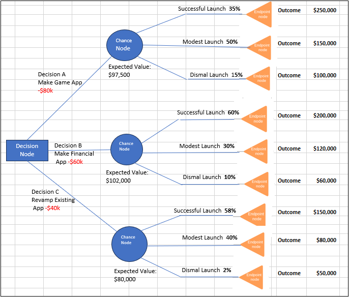
The expected value is shown at each chance node. To understand how the expected value was calculated, look at Tables 3.6–3.8.
As seen in Exhibit 3.17 and Figure 3.54, the expected value for decision A (the game app) is $97,500. To calculate the expected column, take the payoff multiplied by the probability. Next, total the expected column and subtract the cost to develop the game.
Figure 3.54—Decision A: Expected Value of $97,500
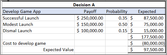
Summary for decision A: ($250,000 × 35%) + ($150,000 × 50%) + ($100,000 × 15%) = $177,500, then subtract the cost to develop the game and you have calculated the expected value for the decision. Notice that .35 + .50 + .15 = 1.00. The probability will always equal 100%.
Figure 3.55—Decision B: Expected Value of $102,000
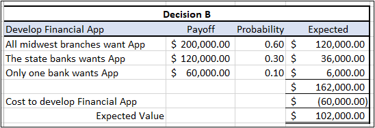
As seen in Figure 3.55, the summary for decision B: ($200,000 × 60%) + ($120,000 × 30%) + ($60,000 × 10%) = $162,000, then subtract the cost to develop the app and you have calculated the expected value for the decision.
Figure 3.56—Decision C: Expected Value $80,000
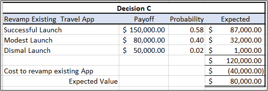
As seen in Figure 3.56, the summary for decision C: ($150,000 × 58%) + ($80,000 × 40%) +($50,000 × 2%) = $120,000, then subtract the cost to revamp the existing app.
Now the three partners of XCaliber Systems sit down and compare the three opportunities. Financially, the best option is decision B, the financial app at $102,000; however, decision A, the game app, is not far behind at $97,500. It is possible that the three partners will still choose the game app, since it is only 4,500 less.
Most decision trees are used where large sums of capital are involved, especially when risk is tied to an external factor that the organization doesn’t control. A good example might be the potential leasing of a venue space owned by an organization for two or more events.
Decision trees are a great way to visualize a complex problem. Risks associated with the problem explored will have already been considered, and visualization facilitates finding the best resolution. In the case of LucidChart, the data are linked to a spreadsheet, and since it was built that way, you can add a button that shows you the best option.
The biggest thing to remember is to show all the probabilities by drawing out each component first. The decision tree yields a visualization comparing two or more projects.
Next, let’s look at another decision-making tool that involves the Pareto Diagram.
Decision-Making Tool #3—How Can a Pareto Diagram Help?
This tool enhances your ability to make informed decisions and has been adopted by many fields, especially in the context of quality management. The Pareto Diagram prioritizes key factors through a visual representation of what industry experts call the 80/20 rule. The typical data used to construct a Pareto Diagram is qualitative data.
To better understand this application, let’s look at an example. POM University purchased an automated system to answer fan questions. The survey had an open-ended question set, and major words were aggregated to show a word cloud. Figure 3.57 shows a summary of the data. These data are set up so we can use a Pareto Diagram. The visualization was sorted from highest to lowest frequency, while a relative frequency column and a cumulative relative frequency column were also added. Notice that some of the phrases relate to the same issue. For example, headache and loud music may relate to the same issue.
Figure 3.57—Data Setup for Pareto Diagram
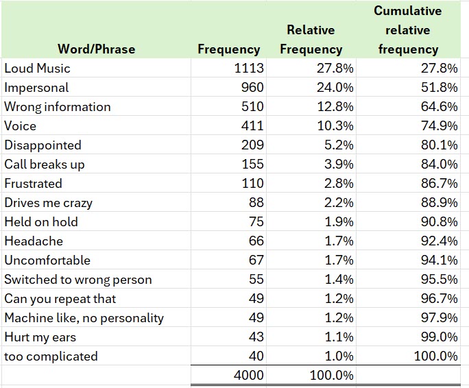
A Pareto Diagram is a bar chart plotted by order of decreasing frequency relative to other data points. In addition to the bars, the cumulative frequency is plotted as a line on the same graph. The line is called the Pareto line. You may have heard of Pareto but didn’t realize it since this graph represents the 80/20 rule. It was named the Pareto Diagram after a well-known Italian economist, Vilfredo Pareto, and is often used in the realm of total quality management (TQM). Exhibit 3.18 shows the 80% components: loud music, impersonal, wrong information, voice, and disappointed. Pareto Diagrams help you concentrate on a few issues to serve the largest number of customers.
Exhibit 3.18—POM University Pareto Diagram
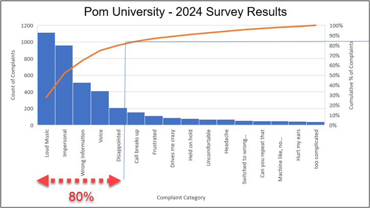
Applying the 80/20 principle to this situation means that 80% of the complaints fall into a few categories. A better way to look at it is that it helps you narrow down the list of complaints that should be prioritized. The Pareto Diagram you see here has a few extra components that we added to draw your eye to where the 80% category lies on the frequency table. Essentially, this means that 3,200 of the 4,000 complaints used these phrases.
Step-by-Step for How to Create a Pareto Diagram in Excel
First of all, a Pareto Diagram is included in the Chapter 3 Excel file “3.4 Survey Data—Pareto Diagram.” You can practice with it.
- Highlight the data but not the totals (B2:E18).
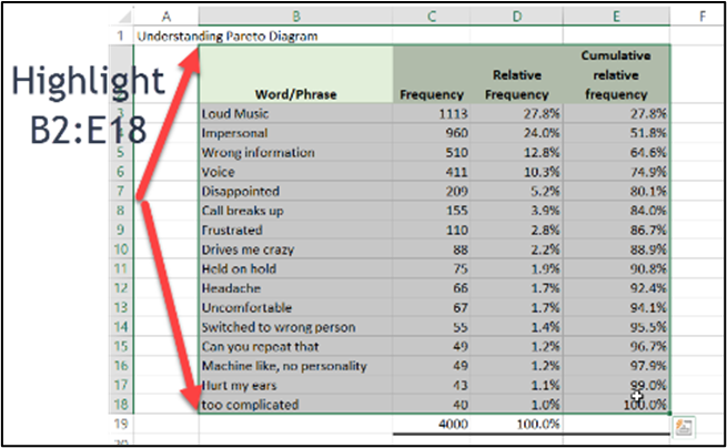
Figure 3.58—Highlighting Area for Pareto Diagram - Choose Insert on the ribbon.
- Look for a small chart icon that when you hover over it is a statistics chart, and then choose the Pareto chart.
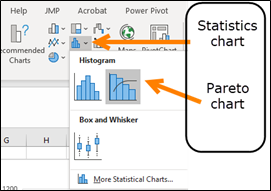
Figure 3.59—Chosing Pareto Chart - Then add some axis titles and a heading.
- Depending on your audience, you can add lines to emphasize the 80% data points as shown in Exhibit 3.18.
- If you plan to use this in a PowerPoint, you may want to highlight the 80% or show an animated arrow.
3.4 Self-Assessment: Use Decision-Making Tools
Learning Objective #5—Create and use decision-making tools to provide context for problems, support decisions, and assess risk
3.5 Self-Assessment: Decision Tree Problem
Learning Objective #5—Create and use decision-making tools to provide context for problems, support decisions, and assess risk
Suppose you have an opportunity to rent out your facility at POM University, but two different organizations want to rent the facility during the same week. As you can tell from reviewing the fact table (Table 3.9), the cost of the bid is nonrefundable.
Table 3.9: Fact Table for POM University Hosting an Event
|
Payoff Table |
Event A |
Event B |
|---|---|---|
|
Cost of bid (nonrefundable) |
$50,000 |
$15,000 |
|
Probability of Organizer choosing your bid |
.30 |
.90 |
|
Costs associated with event in your facility |
$100,000 |
$ 25,000 |
|
Successful hosting |
.60 |
.90 |
|
Not as successful hosting (poor weather) |
.40 |
.10 |
|
Financial benefit if Excellent |
$500,000 |
$150,000 |
|
Financial benefit if weather issues or mediocre competitions |
$400,000 |
$100,000 |
Use LucidChart, Venngage, Canva, Excel, or paper to build the decision tree for POM University. Calculate the expected value to fill in the blank.
Table 3.10: Event A Expected Value
|
Payoff Amounts |
Probability |
Expected Value |
|---|---|---|
|
$ |
|
|
|
$ |
|
|
|
Subtotal |
|
|
|
Cost of Hosting |
|
|
|
Subtotal |
|
|
|
Probability event chosen |
|
|
|
Cost of bidding |
|
|
|
Expected Value and net worth |
|
|
Table 3.11: Event B Expected Value
|
Payoff Amounts |
Probability |
Expected Value |
|---|---|---|
|
$ |
|
|
|
$ |
|
|
|
Subtotal |
|
|
|
Cost of Hosting |
|
|
|
Subtotal |
|
|
|
Probability event chosen |
|
|
|
Cost of bidding |
|
|
|
Expected Value and net worth |
|
|
Now check your answers against the solution in Exhibit 3.19.
Exhibit 3.19—Solution for POM University Decision Tree
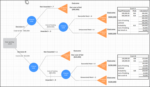
3.4 Exercise 1: Which Event Should Be Contracted for the Convention Center?
Learning Objective #5—Create and use decision-making tools to provide context for problems, support decisions, and assess risk
The exercise assignment is based on the renting of a convention center venue for two potential events: Event A—Girls Volleyball Junior National Championship; or Event B—State High School Coaches Association Convention.
 This exercise (case) was written by Ceyda Mumcu and Kimberly Mahoney and is available in the digital commons (Sports Management Commons) at this URL: https://digitalcommons.newhaven.edu/sportmanagement-facpubs/14/
Reference: Mumcu, C., & Mahoney, K. (2018). Use of decision tree model in sport management. Case Studies in Sport Management, 7(1), 1–3.
Instructions
Take the role of a sports marketing manager. However, please note that the application learned here can be used in any field. The questions for the case have been modified to the following. Complete only these three questions and post your recommendation and support.
- Question 1, modified: Construct a decision tree (using LucidChart, Excel, or Visio). The decision tree can be saved as an image file or screen captured into a Word document or a PowerPoint.
- Question 2: Compare the three alternatives (Event A, Event B, or not bidding for any event) for their expected values and net gains.
- Question 3, modified: Prepare the recommendations—include a five-minute video maintaining your role as the sports marketing manager. Tell the story. Use the decision tree and any other information to make the recommendation.
Make sure to read through the case to consider the context so you can tell the story.
Table 3.12: Payoff Table for Bidding and Hosting Sporting Events
|
Payoff Table |
Event A |
Event B |
|
Cost of Bidding |
$200,000 |
$10,000 |
|
Probability of Being Awarded |
.1 |
.9 |
|
Cost of Hosting |
$1,000,000 |
$60,000 |
|
Probability of Hosting Successfully |
.7 |
.9 |
|
Financial Benefit Expected by an Excellent Event (including revenue for the convention center and economic impact for the city) |
$50,000,000 |
$3,750,000 |
|
Financial Benefit Expected by a Mediocre Event (including revenue for the convention center and economic impact for the city) |
$38,000,000 |
$1,600,000 |
3.5 Visualize and Persuade
An editorial approach to visualization design requires us to take responsibility to filter out the noise from the signals, identifying the most valuable, most striking or most relevant dimensions of the subject matter in question.
—Andy Kirk
Presenting your ideas, research, or insights is a complex endeavor that demands adaptability, empathy, and precision. Whether you are standing before a poster show audience, addressing a small or large gathering, connecting remotely, or speaking to individuals of varying cultural backgrounds or genders, the art of effective communication is a key component that we refer to as “visualize and persuade.”
In an interconnected world where communication bridges gaps and supports understanding, refining these presentation techniques will empower you to deliver compelling messages that resonate, captivate, and inspire, regardless of the context or audience you encounter. Start with something simple, a poster show.
What Is a Poster Show?
A poster show is an event where posters are on exhibition and contain a researcher’s findings, projects, or ideas using a poster as a visual aid. Posters contain visually appealing representations of the subject matter. Posters are often created in PowerPoint, and the sizes include 24″ × 24″ templates to 48″ × 96″ templates and every size in between. (Warning: PowerPoint is limited to 56″ × 56″ in size.) The size depends on the guidelines of the event organizer and whether the presenter wants a vertical or horizontal poster. Attendees can browse through the posters and ask questions to the presenters, and many remote poster sessions include “live” sessions where the presenters put on a short presentation and take questions from the virtual audience. The size shown for Exhibit 3.20 is 24″ × 36″.
The example (Exhibit 3.20) includes the expected components of a virtual poster:
- abstract and title,
- link to presentation video/audio file,
- contact information,
- introduction and hypothesis (if a research poster),
- background,
- methods/results,
- charts or information supporting results,
- more examples to support hypotheses,
- conclusion, and
- references.
Keep in mind to adjust your virtual poster to meet the requirements of the conference or journal.
Exhibit 3.20—Example Virtual Poster.

Poster Checklist
To see if the poster is following best practices, let’s start with a poster checklist (Table 3.13). Use the poster in Exhibit 3.20 and work through the Generic Poster Checklist. Always make sure to review the journal’s submission guidelines in addition to the Generic Poster Checklist.
Table 3.13: Generic Poster Checklist
|
Checklist Questions |
Response |
Explanation as required |
|---|---|---|
|
1. Does the poster meet guidelines or organizer requirements? |
|
|
|
2. Is the message clear and focused? |
|
|
|
3. Does the poster have high-quality images and charts that are engaging without being overwhelming? |
|
|
|
4. Is the poster organized logically, with subheadings, guiding the viewer through the information? |
|
|
|
5. Is the data clear and understandable with good data visualization(s)? |
|
|
|
6. Does the presentation or video (if applicable) engage the viewer? |
|
|
|
7. If questions are asked by viewers, does the presenter add meaningful discussion? |
|
|
|
8. Are there visual cues, with effective use of color, white space, and cohesion? |
|
|
|
9. Is the poster accessible to all viewers, including those with disabilities (like closed captioning for a video)? |
|
|
|
10. Does it contain appropriate branding with contact information if viewers wish to reach out for further discussion? |
|
|
|
11. Does the presenter craft a compelling narrative that takes the viewer on a journey? |
|
|
|
12. Does the poster contain appropriate citations and references? |
|
|
|
13. Does the poster use person-first language and show a sensitivity to potential viewers? |
|
|
Poster Presentation Guidelines
The following guidelines were taken from a graduate certificate in women’s leadership (GCWL) program and modified to include some of the innovative ways to participate in poster shows. Most conferences offer a poster show opportunity, and requirements will vary from one conference to another. Therefore, the requirements listed here are just shown as an example.
Using Posters in a Virtual or Hybrid Setting
Poster sessions can be face-to-face or offered virtually. In this example, Saint Mary-of-the-Woods College (SMWC) partnered with Genigraphics Research Posters to provide a virtual experience. Partnering allowed students to receive feedback in the form of discussion or virtually (through Zoom in breakout rooms). Most often, the conference will provide PowerPoint poster templates and suggest several layouts but with a specific size. In this example, SMWC used Genigraphics Research Posters to provide a rich experience for the poster participants. As shown in Exhibit 3.21, Genigraphics offered a portal for GCWL students to upload their posters in time for a virtual poster show. The audience logged into the Research Posters session to view the poster, leave feedback, or talk to the researcher through Zoom (as shown in Exhibit 3.21).
Exhibit 3.21—Setting Up a Poster Event

Exhibit 3.22—Virtual Poster Show (2021) Through ResearchPosters.com

To understand how this project came together, here are the actual requirements given to students who participated in the poster show.
Exhibit 3.23—Sample Poster Requirements
Poster Format Requirements
- Your poster must meet these guidelines, so please use one of the templates at the link provided through email.
- This is a culminating activity. If you, as the presenting author, cited a disclosure on your disclosure form, please also add this to your poster.
- A section at the top of the poster must contain the Title, Author, and Affiliation.
- Files must be in PowerPoint (.ppt or .pptx) or Adobe Acrobat (.pdf) file format.
- Fonts other than standard Windows TrueType must be embedded in the file.
Poster Templates
- The poster needs to be 24″ × 36″. There are several different template styles and layouts to pick from.
- To see how ePoster files look on www.ResearchPosters.com, review the demo: https://www.researchposters.com/display_posters.aspx?code=DEMO1
- All files will receive a complimentary design review.
Audio File Attachments
- All posters must include a 5-minute audio in addition to the video.
- Audio is limited to 5 minutes. Audio files should be uploaded in .mp3, .wav, or .m4a file formats.
- To record audio on your computer, one option is https://online-voice-recorder.com/, which records in .mp3 and saves to your downloads folder. Another option is to use Windows Voice Recorder.
Video
- Posters are required to have a video URL link on the poster.
- Your video should not exceed 7 minutes.
- To include a recorded video, place a hyperlink to the video site within the poster. Directions for video recording (using ScreenPal) will be provided.
To see some of these, feel free to browse the variety of templates available for you to use at Genigraphics (genigraphics.com) and check out other potential poster guidelines.
Other poster guidelines are available.
Virtual Poster Presentation Guidelines. (2021/22). A Celebration of Scholarship. John Carroll University. https://jcu.edu/sites/default/files/2021-02/Virtual%20Poster%20Presentation%20Guidelines_0.pdf
Poster Presentation Guidelines: Create A Successful Post for Presentation At the Conference. (2023). SPIE. www.spie.org
Center for Teaching Excellence & Innovation. (2022). Effective Poster Presentation. Johns Hopkins University. https://ctei.jhu.edu/wp-content/uploads/sites/61/EffectivePosterPresentations-Handout.pdf
A surprising outcome: For the GCWL poster show, the PowerPoint template requirement was 24″ × 36″, and students were given four different layouts. Surprisingly, students chose only two types of templates: (1) abstract sidebar design with large title space or (2) title-left design. Exhibit 3.24 shows an example for each.
Exhibit 3.24—Template Layouts

3.5 Exercise 1: Create a Poster
First of all, you are not required to “create” a poster. However, you are required to discuss components and consider how you would modify an existing template.
- Look at research poster designs in Canva and Venngage and compare them to those that you see in Genigraphics (https://www.genigraphics.com/templates).
- Download a template and open it in PowerPoint. Conduct some preliminary research on a topic of your choice. This could be organization specific. For example, your topic might be based on a challenge at work (poor communication, multigenerational communication issues, a need for conflict resolution techniques, Zoom burnout, employee retention, and so on). Discuss what headings you would use. What are the key components that would support your topic, and how would you show them?{~?~IM: insert pln-mitchelldeckard-discussionicon here. ALT: TK}
- What data visualizations would you expect for your topic?
Based on your instructor, either post to a discussion board or be prepared to discuss in class.
3.6 Visualization Tools Animated Through Time
Without a systematic way to start and keep data clean, bad data will happen.
—Donato Diorio
We have unprecedented access to data and tools available that will empower us to explore, analyze, and understand the intricate web of global trends with clarity. Hans Rosling once said that people are not “rocks” and that we are transforming. The rapid transformation in economics, demographics, health, and education shows distinct patterns through time. Tools like Gapminder and Flourish empower users to breathe life into static datasets. Both tools engage the viewer and facilitate a deeper understanding of trends and patterns. These types of tools play a pivotal role in transforming raw data into compelling narratives.
Gapminder Tool was developed by Hans Rosling and his team and is an innovative use of data visualization because it combines animated trends into a compelling narrative that reveals the true stories of our world. This tool was introduced earlier in the interactive infographic tools in Chapter 2. In this section, you will explore how to use the Gapminder Offline Tool using your own data.
Gapminder—a Visualization Tool Animated Through Time
If you have data that has years and you want to show the trend over time, this product will fill that need. But before you add your own data, explore Gapminder because the data already collected may offer further insight. Let’s look at the image shown in Exhibit 3.25 and explore some of the options. Notice that this is an animated infographic (see the play button on the bottom left), which can be saved as a video that can be inserted into PowerPoint.
Exhibit 3.25—Gapminder GDP and Life Expectancy
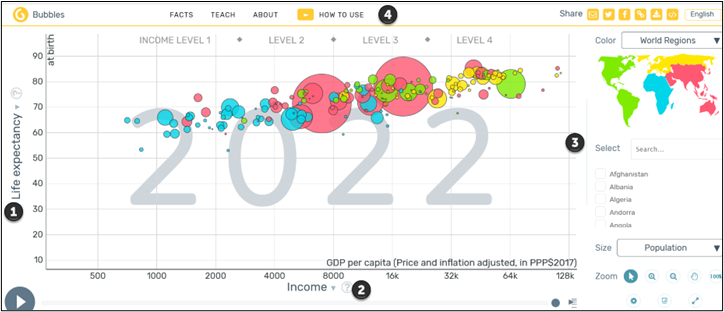
![]() This is the y-axis. Besides life expectancy, there are hundreds of possible choices, by choosing the drop-down arrow and exploring the categories: communication, economy, education, energy, environment, health, infrastructure, population, society, sustainability, work, an advanced user section, and other datasets.
This is the y-axis. Besides life expectancy, there are hundreds of possible choices, by choosing the drop-down arrow and exploring the categories: communication, economy, education, energy, environment, health, infrastructure, population, society, sustainability, work, an advanced user section, and other datasets.
![]() This is the x-axis. Besides income, there are hundreds of possible choices by choosing the drop-down arrow. It includes all the same categories listed for the y-axis and includes data from 1800 through 2020 (when the x-axis is time).
This is the x-axis. Besides income, there are hundreds of possible choices by choosing the drop-down arrow. It includes all the same categories listed for the y-axis and includes data from 1800 through 2020 (when the x-axis is time).
![]() This section gives you the option of filtering the information, making it easy to compare one country to another. But it also has hundreds of options with the drop-down arrow. Note that you can share the video you make through social media options.
This section gives you the option of filtering the information, making it easy to compare one country to another. But it also has hundreds of options with the drop-down arrow. Note that you can share the video you make through social media options.
![]() This menu includes a “How to Use” section. More importantly, it shows directions on downloading the Gapminder Tool and how to use this tool to show your own data.
This menu includes a “How to Use” section. More importantly, it shows directions on downloading the Gapminder Tool and how to use this tool to show your own data.
There is a step-by-step tutorial for showing your own data on the Gapminder website. If you review this section, you will notice that you can choose templates that have bubble charts, bar rank charts, line charts, world maps, and mountains.
Vizabi. (2017, Apr 3). Show your own data. Gapminder Offline. https://vizabi.org/tutorials/2017/04/03/show-your-data/
Flourish—a New Data Visualization Tool for Canva
Note: Screenshots of Flourish interface © Flourish Studio, https://flourish.studio. Used with attribution for instructional and illustrative purposes. Annotations added by the author.
According to Christine Hall (2022), “Canva acquired Flourish in mission to tell better stories with data” (para 1). Canva has a free account available to students and educators. In addition, Canva has many apps that add to its already broad range of infographic and design features. One such app is Flourish. To use Flourish in Canva, you must add it as an app in Canva, set up a new account in Flourish, and connect them. One of the key impacts of Flourish is how the animation can help inform, persuade, and inspire your audience. Before we get to the step-by-step, look at the many types of animated graphs available.
There are three categories of animated templates available in Flourish: (1) line, bar, and pie charts; (2) projection maps; and (3) scatterplots. Exhibit 3.26 shows only a partial list.
Exhibit 3.26—Types of Animated Charts Available in Flourish
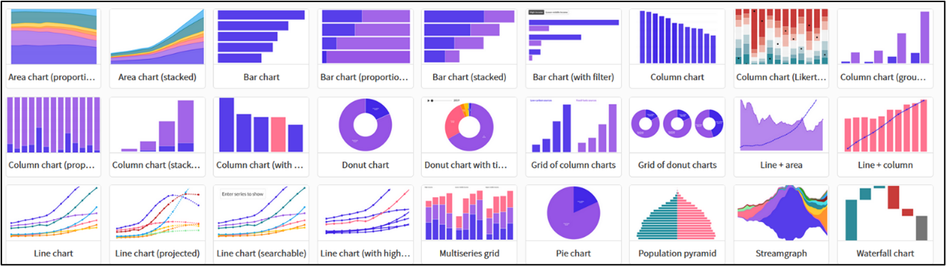
Exhibit 3.27—Types of Animated Maps Available in Flourish
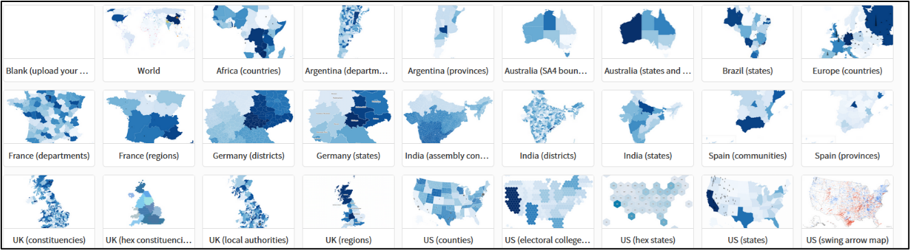
Exhibit 3.28—Types of Scatterplots, Time Sliders, and Minicharts Available in Flourish
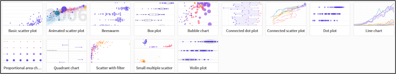
These three exhibits show the depth of available templates to use with your dataset. Now that you know all the potential templates available, get started adding Flourish to your Canva account and using Flourish to create an animated graphic.
Step-by-Step to Use Flourish in Canva
Note: Screenshots of Flourish interface © Flourish Studio, https://flourish.studio and Canva © Canva, https://www.canva.com. Used with attribution for instructional and illustrative purposes. Annotations added by the author.
Exhibit 3.29—Flourish: Example of Setting Up Dataset
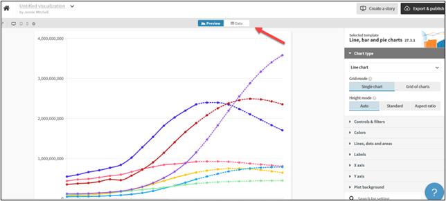
- Log into your Canva account (or set up your free account).
- In Canva, click on the home icon to go to your home screen, click on Apps, and do a search in the search bar for Flourish. Click the red sunburst icon under the search bar (refer to Figure 3.60).
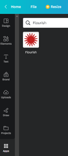
Figure 3.60—Sunburst Icon - This will bring up a “Welcome to Flourish!” account screen. Use the Sign up now button to create a Flourish account. We used the same email account that we had for our Canva account (see Figure 3.61 in step 4).
- Connect the two accounts by choosing Connect.
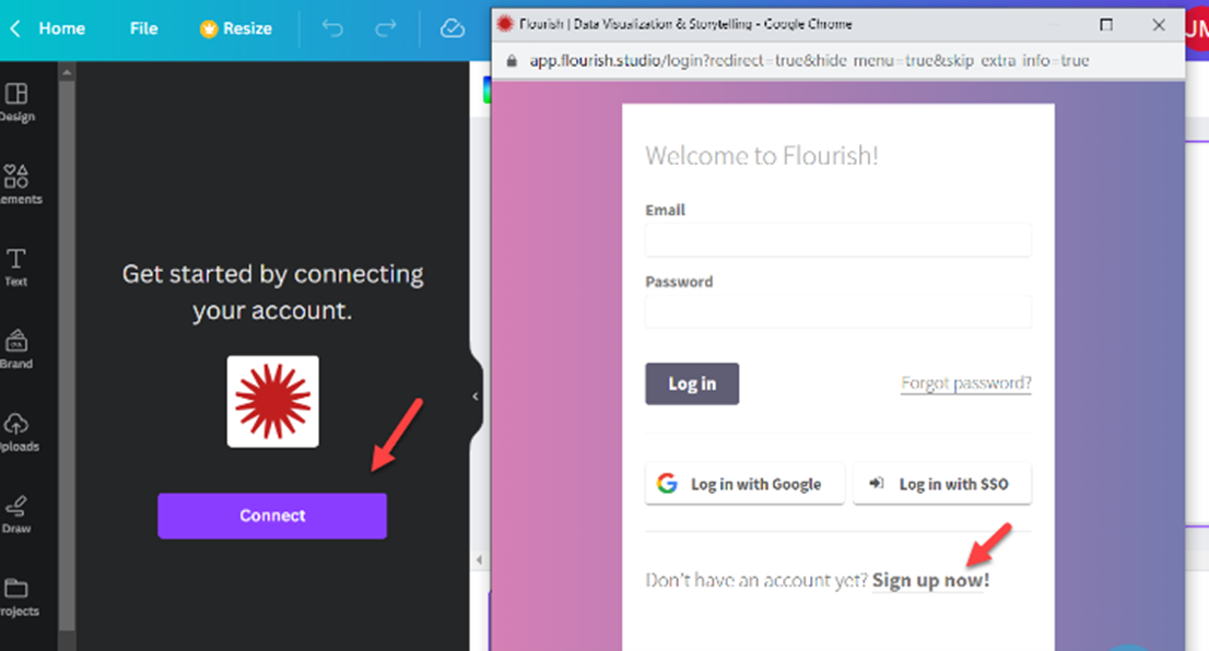
Figure 3.61—Flourish Account Screen - Once you have the two accounts connected, you will see a screen something like the one pictured here. We found it easier to log into our Flourish account, create our animation design, and give it a title. Afterward, the project title can be searched within Canva. If you have not created anything in Flourish, it will not show up as depicted in Figure 3.62.
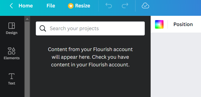
Figure 3.62—Empty Flourish Content - We selected a projected line chart because we wanted to use some information about women leaders in the United States and later compare it to women leaders in other countries. The template comes with example data so you can see how it works and replace it with your own.
One thing to note: The data required some cleaning because when there was no change in leadership percentage (because of periodic elections), the Pew Center dataset skipped the year. We had to make sure there were no missing years of data. Here is the link to the data: https://www.pewresearch.org/social-trends/fact-sheet/the-data-on-women-leaders/ Also, when you first arrive at “The Data on Women Leaders,” the charts are in graph form. Notice at the bottom right of each graph a way to link to the data as shown in Figure 3.63.
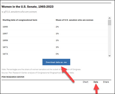
Source: Screenshot of Women in the US Senate, 1965-2003 © Pew Research Center. Author Annotations Added
- We found information about women leaders in the United States at the Pew Research Center (2021). We chose data from 1995–2019 and replaced the template data with our own data named “Women Leaders in the U.S. (1995–2019).” There is a place to upload a data file, but we just typed it into Flourish (Figure 3.64).
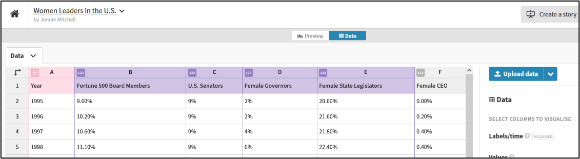
Figure 3.64—Women Leaders in the U.S. (Pew Research Center) - Next, we previewed the data, which included a full preview with animation in a new window. The animation was too fast. When presenting this data and telling a story, you want the audience to be able to see the animation. On the right-hand side of the line chart, there are all kinds of controls. We selected Animations and changed the animation to 2,700 (the default was 900).
- Next, we added a large title on the graph, “Women Leaders in the U.S.,” and a subtitle, “1995–2019.”

Figure 3.65—Creating a Story and Adding a Caption - Next, you can select Create a Story and add a caption (shown in Figure 3.65). We added a quote from U.S. Senator Joni Ernst (visible in Exhibit 3.30).
- You have several options at this point. Choose Publish to share and embed, and a pop-up will display this message: This project will be published to its own page where you and others can see, share and embed it.This option works well if you have multiple ways you want to use this. (Feel free to visit the URL and see this animated line chart. You can see the URL in Figure 3.66.)
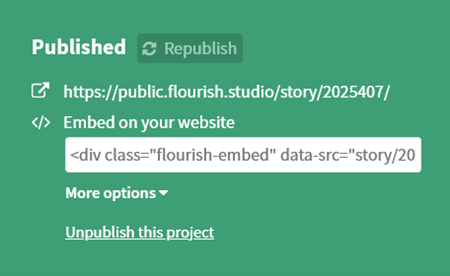
Figure 3.66—Option 1: Publish to Share and Embed - You can choose Add to Canva presentation, which will bring up an untitled presentation with a place to add the animated line chart. This is the best option if you are making a presentation on this topic.
- Do not choose “Download HTML” because it is not available for the free account.
Exhibit 3.30 illustrates the final product. If you go to the URL, you will see the animation. Link to URL: https://public.flourish.studio/story/2025407/
Exhibit 3.30—Women Leaders in the U.S., as Shown in Flourish
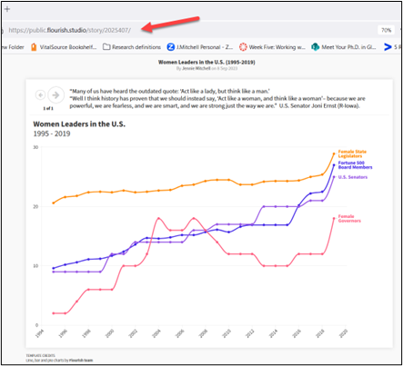
You may be thinking, “I can do this in PowerPoint!” While PowerPoint’s animation capabilities allow you to create dynamic and visually engaging chart series, it’s important to note that Flourish offers more advanced features, interactivity, and customization options specifically designed for data visualization. The combination of Flourish and Canva will allow you to combine the interactivity of Flourish with good design presentation templates available in Canva.
3.6 Self-Assessment: Insightful Tools
Learning Objective #1—Determine insights
Learning Objective #5—Create and use decision-making tools to provide context for problems, support decisions, and assess risk
3.7 Data Visualizations Used in Statistics
In school we learn a lot about language and math. On the language side we learn how to put words together into sentences and stories. With math, we learn to make sense of numbers. But it’s rare that these two sides are paired. No one tells us how to tell stories with numbers. . . . This leaves us poorly prepared for an important task that is increasingly in demand.
—Cole Nussbaumer Knaflic
In our data-driven world, the sheer volume of information at our fingertips can be overwhelming. In this era of abundant data, the ability to make sense of it all, draw meaningful conclusions, and make informed decisions has become a fundamental skill across various domains. Data visualization stands as a powerful ally in this quest for understanding, as it allows us to transform complex datasets into clear, engaging, and actionable insights. In this section, we embark on a journey through the multifaceted landscape of data visualization, exploring how it aids our comprehension of descriptive statistics, inferential statistics, Six Sigma, exploratory data analytics, causal analytics, and predictive analytics.
There are specific guidelines for how statistical data are presented, but it is the data visualizations that help the researcher grasp the central tendencies, variations, and shape of the data distribution. Whether it’s a histogram depicting the frequency of values or a box plot revealing the spread of data, these visualizations breathe life into statistical summaries. An analytic journey can help answer the questions, What happened? Why did it happen? What will happen? and What should be done about it? Exhibit 3.31 of the analytic journey shows how these questions are answered.
Exhibit 3.31—Analytic Journey: How the Questions Are Answered.
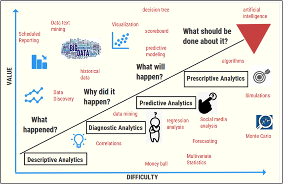
Descriptive Statistics
Descriptive statistics should be a first step in an analytic journey. At the heart of the exploration is an initial recognition that diverse types of data lend themselves to different visual representations. Some of this has been highlighted in previous chapters, but this section takes it a step further. In the quest to understand which visualization illuminates descriptive statistics, keep in mind that this text will always focus on understanding through visuals, so if the word statistics makes you uneasy, take a breath and be assured that you do not have to understand the math behind the statistics. Instead, the visuals will lead you to the correct decision! So what are descriptive statistics?
Descriptive statistics describe and summarize the data and display characteristics of the location, spread, and shape of the data. Through visuals, you can describe a trend or specific features. Tools used to visualize descriptive statistics include bar charts, pie charts, histograms, scatter graphs, box plots, and more. Descriptive statistics address the question, “What happened?” Numerical descriptive tools allow you to summarize data for average, mean, mode, minimum, and maximum. There are two types of statistics used to describe data:
- the measure of central tendency (mean, median, or mode)
- the measure of spread through range, quartiles, variation, and standard deviation
So far, the explanation has used only words. Dive into an example to see what visuals can do to help you understand.
Example Scenario: Measure of Central Tendency—Finding the Mean and Median
The data in Figure 3.67 shows crime data reported on 14 college campuses. Everything listed here is fictitious. Notice that the crimes range from 0 to 29 and that the student population ranges from 692 to 47,993.
Figure 3.67—Fictitious Crime Data at 14 College Campuses
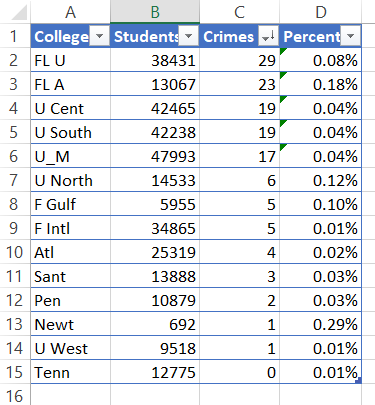
You can tell it has been formatted as a table by the drop-down arrows. It has also been sorted from highest to lowest by the number of crimes. The percentage was an added calculation.
The mean (arithmetic mean) is the average of the values or the “center” of the data. In this case, the mean can be calculated using Excel using the =Average (B2:B15) or (22,330) for the mean of the number of students and =Average (C2:C15) or (9.6) for the mean of crimes.
The median is the midpoint of a set of data values when you put them in order (either smallest to largest or largest to smallest). It always splits the data into two equal halves. Using Excel, the formula is =median (B2:B15) or (14,211) for the number of students and =median (C2:C15) or (5.0) for the crimes.
You may be asking yourself,
Why is the mean for crimes (9.6) so different from the median (5.0)?
It could be due to outliers. Outliers are values much larger or much smaller than the rest of the values. Outliers don’t have much impact on the median, but outliers can have a drastic effect on the mean. Since the mean is the balance point, extreme values in the data will pull the mean toward it to maintain the balance (see Exhibit 3.32 to see the balance point).
Exhibit 3.32—Understanding Mean and Median
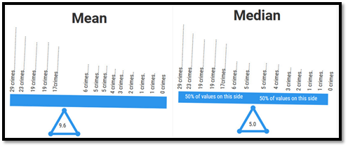
Example Scenario: Finding the Mode
To find the mode (or modal value), put the list in order. Then count the quantity of each number. The number that appears most often is the mode. It is possible to have more than one mode. Two modes are called bimodal, and more than two are called multimodal.
In Excel, there are several formulas for calculating mode. Look at the data again. You can see two 19s, two 5s, and two 1s. So these data are considered multimodal (see Table 3.14).
Table 3.14: Multimodal and Mode
|
Excel formula for multimodal |
Excel formula for single mode |
|---|---|
|
=MODE.MULT(C2:C15) This will show 19, 5, and 1 |
=MODE (C2:C15) This will show you just the value 19. |
Now let’s look at a visual (histogram) of this data. The taller “peaks” of the histogram indicate where more common data values cluster. These are the modes.
A histogram is a visual of the modes, but it can look different depending on the number of bins (or how you cluster your data). Notice in Exhibit 3.33 that a normal curve serves as a guide to measure central tendency. Central tendency is the statistical measure that best represents the value where all the other data gather. If you don’t see that in this example (and you don’t), that means these data are not on a normal distribution. It is skewed because one side has more data than the other. A normal distribution, called the bell curve or Gaussian Distribution, is a continuous probability distribution that is symmetrical. Keep in mind that the sample is only of 14 college campuses.
Exhibit 3.33—Histogram in Statistical Package for Social Sciences (SPSS)
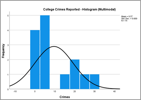
You can create a histogram in Excel as shown in Exhibit 3.34. In this example, a bin size of 3 was used. You can click on the axis and adjust the bin size. Graphing the data makes it easier to see that the data are multimodal.
Exhibit 3.34—Histogram in Excel
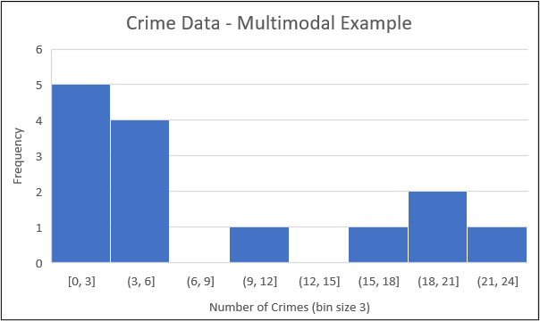
So the visual that might be more explanatory is a “dot plot.” Note that you see the multimodal pattern of 1, 5, and 19. Make sure to compare the dot plot (in Exhibit 3.35) to the previous histogram.
Exhibit 3.35—Dot Plot of Crime Data
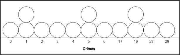
Another visual often used (especially in a business setting) is a box plot. A box plot is a visual of the variables, distribution location, spread, shape, tail length, and outliers. It is sometimes called a box and whisker plot. The box spans the interquartile range (IQR) of the data and represents the middle 50% of the dataset. The IQR includes the first quartile (Q1) and the third quartile (Q3). The whiskers extend from the box to the data points outside the IQR.
How to Interpret a Box Plot
- Central tendency: If the median is near the center of the box (the example is not), the data are roughly symmetric; if it’s closer to one end, the data may be skewed.
- The length of the IQR illustrates the data’s range. A longer box indicates greater variability, while a shorter box suggests more consistency.
- There are no outliers in this example, but if an outlier existed, it would show as a data point beyond the whiskers.
Figure 3.68—Box Plot of Crime Data (Prepared in Excel)
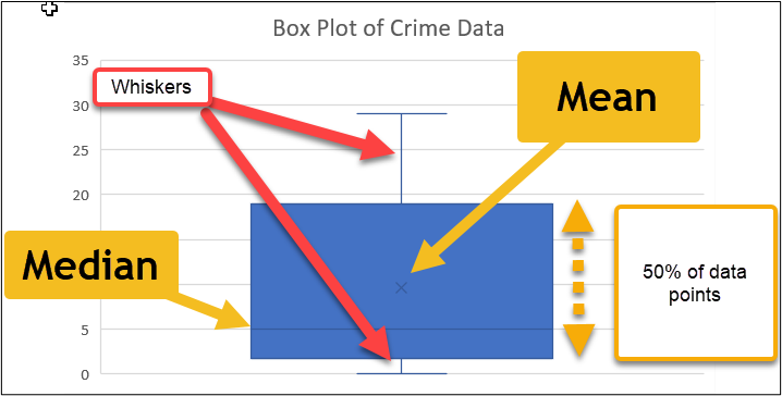
The example of the box plot created in Excel (Figure 3.68) shows a vertical format. It is possible to create a horizontal box plot in Excel, but it requires multiple steps. Instead, Figure 3.69 shows how to create the box plot in Statistics Kingdom (an online and free statistics helper). It is much easier to see how the data are skewed when viewing in horizontal format.
Figure 3.69—Box Plot of Crime Data (Prepared in Statistics Kingdom)
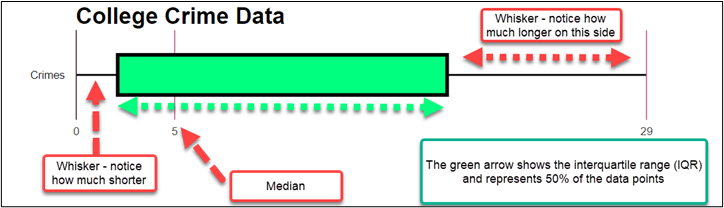
You may want to bookmark the Statistics Kingdom website. It is easy to use and models example data points, so you see how to set it up. As previously mentioned, it is possible to change the layout to a horizontal box plot instead of a vertical box plot. We find this layout easier to understand. Statistics Kingdom has several visualization choices: histogram, box plot, violin plot, cluster analysis chart, Venn diagram, stem-and-leaf plot, and more.
Statistics Kingdom. (2017, November). http://www.statskingdom.com
Analyze Data in Excel
In the more recent Microsoft 365, you will see an icon in Excel on the home screen renamed Analyze Data. According to Microsoft, “Analyze data in Excel empowers you to understand your data through natural language queries that allow you to ask questions about your data . . . [providing] high-level visual summaries, trends, and patterns” (Excel for Microsoft 365, 2023, para 2).
Here’s how to use the new tool:
- Click inside the data.
- On the Home tab, select Analyze Data.
- Browse through the various ways to Discover Insights.
- In Figure 3.70, one of the insights found shows that there is a correlation between students and crimes, but don’t start making assumptions. This is a small sample and there are likely other variables that impact the data. This is a scatterplot chart; notice the clustering of the data points (correlations will be further discussed in the inferential statistics section). But still, this new AI feature is powerful!
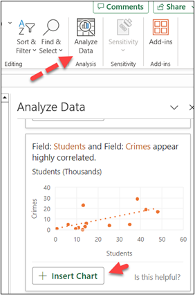
Figure 3.70—Analyze Data Feature in Excel
Source: Screenshot of Excel Interface © Microsoft Corporation. Author Annotations Added
Descriptive Statistics and Add the Analysis ToolPak in Excel
Before you can do anything with statistics in Excel, you need to add the Analysis ToolPak as an add-in to Excel. Here are the steps to add it.
Step-by-Step to Add Analysis ToolPak in Excel
Note: Screenshots of Excel interface © Microsoft Corporation, used with attribution for instructional and illustrative purposes.
You first need to make sure you add the Analysis ToolPak (and solver) in Excel. Macs have access to these tools, but the following steps are for a PC.
-
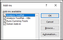
Figure 3.71—Select All Tools Click the File tab, click Options, and then click the Add-ins category.
- In the Manage box, select Excel Add-ins and then Go.
- In the Add-ins box, check the Analysis ToolPak check box, and then OK.
- Select all the tools (see Figure 3.71).
- Once you have this added, it should appear on your ribbon in the Data tab.
Figure 3.72—Data Analysis Tools Available in Excel - Open the Data Analysis tools, you will be amazed at the number of tools packed into Excel! See the partial list in Figure 3.72.
There are several reasons why a decision-maker would want to run descriptive statistics. Descriptive statistics will summarize the data. The data visualizations that accompany this step (histograms, box plots, dot plots) help decision-makers interpret the data more intuitively, identify trends, and spot outliers or unusual patterns. Descriptive statistics measure central tendency (mean and median), measure dispersion (range, standard deviation), and help decision-makers understand the variation and spread of data.
This type of understanding is crucial for assessing the consistency and predictability of outcomes. Although not discussed yet, descriptive statistics can help through metrics like mean and standard deviation for quality control. Even with the small College Crime dataset, it shows that crimes are reported more often if your student population is smaller. Although our sample is too small to make this statement with certainty, it is possible that this might be a starting point for hypothesis generation. So let’s run the descriptive statistics using Excel.
Step-by-Step to Generate Descriptive Statistics in Excel
Use the Descriptive Statistics worksheet in Chapter 3, and follow these steps:
- Click somewhere inside the College Crime dataset (see Table 3.11 for the raw dataset).
- Select the Data tab and click Data Analysis.
-
Figure 3.73—Descriptive Statistics in Excel
Source: Screenshot of Excel Interface © Microsoft Corporation.In the pop-up window, select Descriptive Statistics and click OK.
- A pop-up window will appear. The input range should be the students column and the crimes column (B1:C15). You can use the headings as long as you check the “Labels in first row” box (see Figure 3.73 showing the checkbox checked).
- There are several places to output the data. If you want it on the same sheet, make sure to give it plenty of room.
- Also check the “Summary statistics” box.
- And the last step, click OK.
You may want to watch this short video to see a demonstration of Descriptive Statistics in Excel.
Mitchell, J. (2021, Mar 30). Descriptive statistics in Excel [Video]. YouTube.
Now let’s look at what Excel gave us for descriptive statistics. We’ll go through each term. Some of these terms should look familiar.
Terms of Descriptive Statistics
- Mean—an average of the numbers
- Standard error—measures the accuracy with which a sample distribution represents a population by using standard deviation
- Median—exact middle of the set of values
- Mode—the most frequently occurring value. This dataset has three numbers that repeat (19, 5, and 1). Therefore, it is considered multimodal.
- Standard deviation—an estimate of the dispersion. Remember, an outlier can greatly exaggerate the range.
- Kurtosis—refers to the degree of presence of outliers in the distribution
- Skewness—a measure of the asymmetry of the distribution. You may have seen this drawn by a professor when they were explaining the bell curve.
Exhibit 3.36—Example Showing Descriptive Statistics in Excel
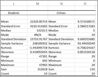
There are three types of skewness:
- a positive skew (long right tail),
- a symmetrical distribution (the bell curve or the normal distribution), and
- a negative skew (long left tail).
In a normal distribution, the tails on either side of the curve are exact mirror images of each other. In Exhibit 3.37 the histogram of the College Crime dataset shows a positive skew, or long right tail.
Exhibit 3.37—Positive Skew in Histogram for College Crime

In summary, descriptive statistics serve as a critical tool for decision-makers to gain a comprehensive understanding of their data. Now we’ll discuss inferential statistics and look at the difference between diagnostic analytics and inferential statistics.
Inferential Statistics Versus Diagnostic Analytics
Inferential statistics takes the boundary a large step beyond descriptive statistics. It includes hypothesis testing, confidence intervals, regression analysis, and more. It is different from diagnostic analytics. Diagnostic analytics’ goal is to understand why something happened. It aims to identify the root causes of past events or trends. Why did sales decline? Why did enrollment drop? Diagnostic analytics works with historical data and focuses on analyzing events that have already occurred. Diagnostic analytic techniques include drill-down, data discovery, data mining, and correlations. As you might expect, the health care industry uses this analytical model every day. A sudden spike in the emergency room count could be pointing to an infectious agent that has broken out in your area (think of COVID-19!).
The questions often asked for inferential statistics might be “How likely . . . ?” or “What will happen . . . ?” Inferential statistics can be applied to both historical and future data to project estimates. Inferential statistical techniques provide insight to help the decision-maker arrive at a deduction or conclusion. Inferential statistics is a technique that allows us to draw inferences or conclusions about the population from the sample. The tools used most often include hypothesis test statistics (e.g., t-tests, ANOVA), though some of the concepts are beyond this text. However, not all are. So look at the type of data visualizations used in inferential statistics.
You can still expect to see histograms, box plots, and scatterplots as some of the first steps because you should always conduct descriptive statistics to understand your data. Other types of tests could be probability plots, residual plots, time series plots, and many others.
Making a Scatterplot That Tells a “Clear” Story
One of the main visuals in the inferential statistics realm is a scatterplot, which is valuable for visualizing the relationships between two continuous variables. Sometimes you expect a relationship, and the scatterplot will tell you if there is a correlation (or relationship). To understand the use of scatterplots, look at the relationship between perceived astringency and tannins in red wine as illustrated in Exhibit 3.38. Astringency is a term associated with puckering or a drying feeling in the mouth caused by the presence of tannins in wine. Tannins are primarily from grape skins, seeds, stems, or even oak barrels. In a technical brief by Kennedy et al. (2006) in a wine publication, the researchers found a correlation between tannins and astringency.
Exhibit 3.38—Positive Relationship Between Tannins (x) and Astringency (y)
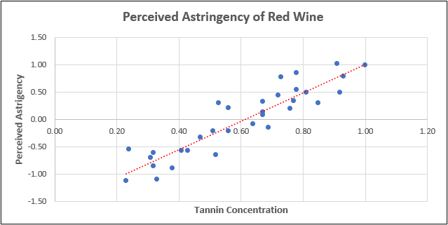
Once you see a linear relationship, it’s time to take the next step, and that is to run a regression to measure the amount of correlation. Regression analysis is an inferential statistical tool. At its core, regression analysis seeks to answer one fundamental question: How does change in one (or more) independent variable influence a dependent variable? In this case, we want to measure the amount of astringency that is caused by tannins. Most wine-tasting experts use their perceived taste to assess whether a wine’s tannins are acceptable in its current state or whether it would benefit from further aging to soften the astringency. But what if you could predict the degree of astringency with a certain level of tannins? Here are the steps using the Tannins and Astringency dataset.
Step-by-Step to Run a Regression Analysis in Excel
Before you can do anything with statistics in Excel, you need to add the Analysis ToolPak as an add-in to Excel. This was shown earlier in this section.
- Open “3.7 Scatterplot and Regression” in Chapter 3 Excel files.
- Click inside the dataset.
- Choose Data on the main menu tab.
- Click Data Analysis and select Regression from the pop-up Data Analysis tool.
- Click OK.
- For the input Y range, choose the perceived astringency column and for the X range, choose the tannin concentration (see Figure 3.74).
- The output range can be a new worksheet, but I chose to run the regression and placed it in the existing worksheet.
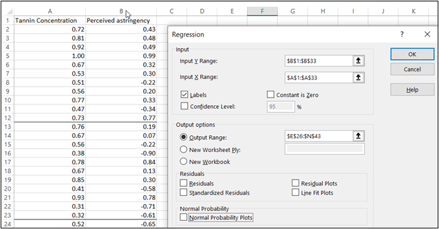
Figure 3.74—Running Regression in Excel
Source: Screenshot of Excel Interface © Microsoft Corporation - Then click OK, and you will see the output as shown in Figure 3.75.
In the illustration, you will notice that there is an equation that should be slightly familiar to you. This regression line is a fundamental component of regression analysis to help understand the relationship between two variables: One is the dependent variable, and one is the independent variable.
The formula is Y = a + b(X), where
- Y represents the dependent variable, the one you’re trying to predict (the perceived astringency);
- X represents the independent variable, the one you are using to make the predictions (this is the tannin concentration in this example); and
- a is the intercept, where the regression line crosses the y-axis.
Figure 3.75—Regression Output for Tannins and Astringency
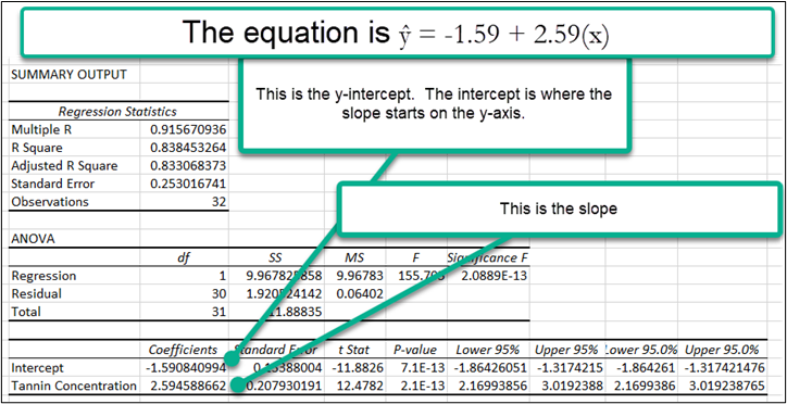
Let’s start by demystifying all the terms.
Regression Terms
Multiple R: This is the correlation coefficient. A value of 1 means a perfect positive relationship. A value of 0 means no relationship, and a value of −1 means a perfect negative relationship. Correlation tells you the degree (or strength) to which two variables move in relation to each other. Correlation measures association but not causation. In this scenario: .915670936 represents a highly positive correlation (which is what our scatterplot showed us).
R Square: This is called the coefficient of determination. It tells you how many points fall on the regression line. In this example, 84% of the values fit the model.
Adjusted R Square: This adjusts for the number of terms in a model. You would use this if you had more than one x variable.
Standard Error: First of all, this is not the same as the standard error in our descriptive statistics! This standard error is about precision. Essentially, this model predicts a variation around the regression line of 0.253016741.
ANOVA: If you are doing basic linear regression (and we are), this section can be skipped. But just so you know what these things are, here is the list:
The df is the degrees of freedom (the sample minus 1). The SS equals Sum of Squares. The MS is the Residual SS / Regression degrees of freedom. F tests for the null hypothesis. Significance F is the significance associated with the p-value (if you look, you will see the same value in the third section under p-value). When you first see this, you may not know what the “-13” means. Just know that it means that it is significant.
Regression Coefficients
We get to the most important part in the regression coefficients section. First let me talk about the linear regression equation.
Table 3.15: Regression Coefficient Formula With Coefficients
|
|
Coefficients |
|---|---|
|
Intercept |
−1.590840994 |
|
Tannin Concentration |
2.594588662 |
Equation: ŷ = a + bx
For our scenario: ŷ = −1.59 + 2.59 (x)
Where b = slope (2.59), where x = the concentration of tannins, and where a = the intercept −1.59
The intercept is where the slope starts at the y-axis. So a wine with a tannin concentration of .5 would predict a perceived astringency of −0.295.
Plugging into the formula would give us the following:
ŷ = −1.59 + 2.59 × (.5) = −0.295
Regression should not scare you! And remember, you realized there was a correlation between tannins and astringency from the visual. The regression just puts numbers to the degree of correlation and gives you an inferential statistic tool to determine astringency if the level of tannin concentration is known!
So how else are scatterplots used?
Scatterplots That Show a Pattern
There are many uses for scatterplots beyond showing a correlation. For example, some scatterplots show a pattern but not a correlation. To demonstrate such a scatterplot, a dataset was downloaded from The Human Development Center (http://hdr.undp.org/en/data), part of the United National Development Programme. Statistical reports are available with over 150 global indicators that can be analyzed in different combinations. Each tells a story. To show some specific tips regarding data with outliers, a small 2020 dataset with 40 countries (as shown in Figure 3.76) was downloaded with the following categories: Internet, GDP, CO2, Cellular, Fertility, and Literacy. For this example, we can create a scatterplot to show the country (Column A) and fertility (Column F) of the 39 countries in 2020.
Figure 3.76—Human Development Center Data
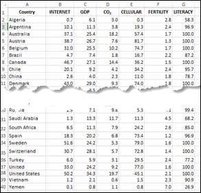
Here are the steps to create a scatterplot:
- Click inside the dataset located in the Chapter 3 Excel file named “Scatter Plot Pattern.”
- Select Insert on the main menu and choose the scatter chart (Excel will try to show you ALL the datapoints).
- Choose Select Data and uncheck all categories except FERTILITY Source, as shown in Figure 3.77.
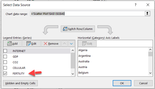
Figure 3.77—Select Fertility Only
Source: Screenshot of Excel Interface © Microsoft Corporation. Author Annotations Added - Click OK.
The default scatterplot will look like Example A in Exhibit 3.39. The red arrow (added manually) indicates an easily spotted outlier. But how could you improve the visual to tell the story better? Improve the title, add a band of color (manually), and add axis titles. Which example contributes more to your story? By using an overlay, we see the outliers more clearly. Example B is formatted so the x-axis shows the number of children, and the y-axis shows the countries.
Exhibit 3.39—Ways to Improve Scatterplot Interpretation
| Example A—Simple Scatterplot | Example B—Improved Scatterplot |
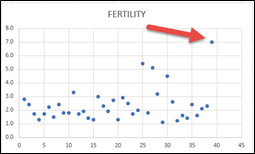 |
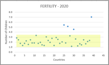 |
| Default scatterplot prepared in Excel, added red arrow manually | Updated title, axis labels, and overlay (yellow highlighting) added manually in Excel |
Let’s assume while you are presenting, you receive a question from the audience:
“What countries are included in this Fertility scatterplot?”
Remember, we have 39 countries in the dataset, but both SPSS and Statistics Kingdom will bunch countries together if they have the same fertility rate. Instead, you can use a bar graph in Excel. As shown in Exhibit 3.40, the red arrow was added manually to the chart image.
Exhibit 3.40—Showing a Bar Graph So Audience Can See All 39 Countries
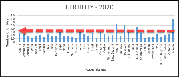
Creating Maps
One of the new features in Microsoft Excel is creating a map chart across geographical regions. This is one of my favorite charts and it’s always been available in Power BI. In the Chapter 3 Excel file, choose the Scatter Plot tab. The dataset shows 40 countries with information about the internet, GDP, CO2, cellular, fertility, and literacy. Exhibit 3.41, shows what a “map” might look like. So the next step is to construct one.
Exhibit 3.41—Using Maps in Excel to Show Internet Speed
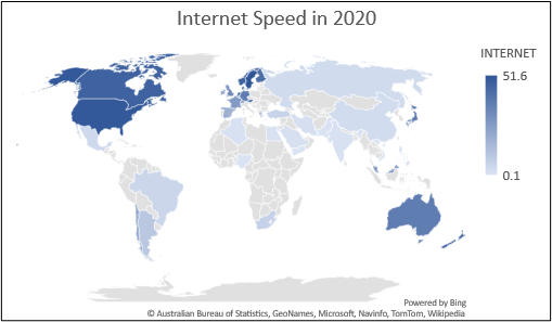
Step-by-Step Instructions to Create a Geographic Data Map in Excel
Before you can do anything with statistics in Excel, you need to add the Analysis ToolPak as an add-in to Excel. This was shown earlier in this section.
- Go to the Scatterplot tab in the Chapter 3 Excel file.
- Next, click inside the dataset.
- Highlight the Country and the Internet columns (A1:B40).
- Choose Insert from the main menu.
- Choose Maps on the Insert menu. See the arrow shown in Figure 3.78.
Figure 3.78—Maps in Excel Icon
Source: Screenshot of Excel Interface © Microsoft Corporation. Author Annotations Added - In the pop-up menu, choose Filled Map.
- Now add a title and you’re done!
Heatmaps and Correlation Matrix
A good visual cue is a heat map. A heatmap is a graphical representation of data by color and it is a great tool for large datasets. For example, heatmaps are often used to show airplane delays, ranging from green for on-time landing, to bright red for delays as much as 40 minutes. Some organizations use a heat map to show website traffic by time of day.
It is also a great way to see if two different groups are on the same page (like CEOs and board members shown in Table 3.16). The images in Table 3.16 show the responses of CEOs and board members who were asked the same questions. The board members saw only a moderate correlation (.6817) for Question 1 with Question 2. The next value is .5633 when comparing Question 1 and Question 15.
But when you look at the CEOs’, there is mostly very high correlation and high correlation with a majority of questions. In fact, on the CEOs’ survey data, only Question 9 had no correlation with other questions.
Correlation is not causation, but it is clear that board members and CEOs are not on the same page. A correlation at .9 to 1 (100%) is very highly correlated, .7 to .9 is highly correlated, and .5 to .7 is moderately correlated.
Table 3.16: Heatmap Shows That Board Members and CEOs Are Not on the Same Page
|
Board members |
CEOs |
|---|---|
|
Question 1 is moderately correlated with Question 2 and Question 15. |
Very high and high correlation throughout. |
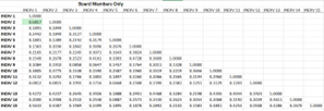 |
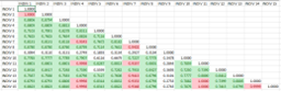 |
A heatmap reduces mental processing because the color saturation provides visual cues. Table 3.16 shows low correlation on the left, indicated by the lack of color and strong correlation on the right indicated by color cues. For this example the numbers are not important.
A heatmap can be produced in Excel using conditional formatting. Creating a correlation matrix is available in Data Analysis (an add-in to Excel) to the Data table. Then you can set up conditional formatting. Compare the two. On the right, which reflects employees, notice how you only see one correlation between Question 1 and Question 15. But if you look at the administrators (CEOs in Table 3.16) answering the same question you see that almost all questions are correlated: Red = very high correlation, and Green = high correlation.
Without the context of the questions asked to both groups, it is difficult to tell the story. But it is clear that the board members and CEOs are not in agreement.
Heatmaps are not just a tool for business. The sports industry uses heatmaps in other ways that you might not consider. Sports team coaches use heatmaps to visualize a team’s player positions, “movement, movement patterns, event occurring spots (events may include penalties, call for foul play, injuries, goals, and so on)” (Khongthaw, 2020, para. 7).
Heatmaps used for large datasets can be somewhat overwhelming. For example, the United Nations Department of Economic and Social Affairs uses a heat map to show supplementary graduation indicators and time series estimates of the least developed countries. The heatmap looks like a quilt with shades of blue, orange, and tan, but just the image provided would take over three pages in a printed textbook to show it!
United Nations: Department of Economic and Social Affairs, Economic Analysis. (2023). Supplementary graduate indicators (SGI) dataset (2002–2023). https://www.un.org/development/desa/dpad/least-developed-country-category/ldc-data-retrieval.html
Link to image of heatmap: https://www.un.org/development/desa/dpad/wp-content/uploads/sites/45/Heatmap.png
Risk Matrix Heat Map
What is a risk matrix? Essentially, a risk matrix is a visual where the organization assesses its exposure to types of harm and plots this information on a risk matrix. The matrix is then used to develop management strategies and implement actions that manage the risk. The risk matrix should consider all the risks associated with an organization including financial risk, operation risk, workforce risk, client (customer) risk, and reputational risk, and in the case of a not-for-profit organization (NFP), programmatic risks. The example shown in Exhibit 3.42 was created in Excel and is included in the Chapter 3 files. This is only an example. If you do a search on a risk matrix, you will see slightly different theories on how the legend and colors would be assigned. Make it your own for your organization. The main point is to consider all the risks your organization faces in the next year and use this matrix to prioritize them. Next, devise strategies that will reduce or neutralize the impact of the potential risks. Remember, each organization is unique; an event that might be catastrophic for one organization might be an acceptable, easily managed risk for another.
Exhibit 3.42—Risk Matrix Heat Map—Blank
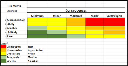
Six Sigma
Inferential statistics are a big part of Six Sigma. Shown in Exhibit 3.43, we see the empirical rule of standard deviation at one (68.2%), two (95.4%) and 3 (99.7%). Six Sigma takes it much further by working with up to 99.9999998% data points, which is ± six standard deviations from the mean.
Exhibit 3.43—Empirical Rule of Standard Deviation.
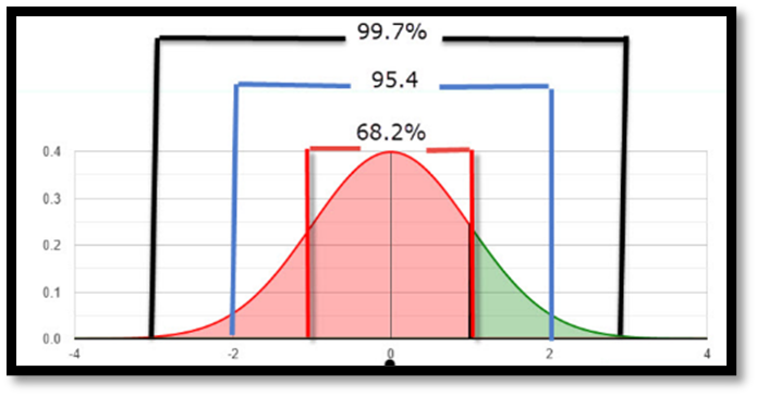
According to Master of Project Academy, “Six Sigma is about creating a culture that demands perfection and that gives employees the tools to enable them to pinpoint performance gaps and make the necessary improvements using data-driven problem-solving methods” (para. 10). Academic researchers are less likely to work with data that requires this level of focus on acceptable levels, but practitioners might be required to work with the Six Sigma model. For example, the quality of a new drug would require this model for quality control.
The DMAIC (Six Sigma) approach to solving a problem includes the following steps: define, measure, analyze, improve, and control. There are a variety of problem-solving methodologies in the corporate setting used to drive quality.
Creating a Six Sigma flowchart in Microsoft’s Visio is easy since there is already a “House of Quality” template available as illustrated in Figure 3.79. The prebuilt house provides rows and column labels, and the roof is the correlation matrix. If this is something you have an interest in pursuing, the YouTube link for a Quality Function Deployment is a good place to start.
Mister Simplify. (2023). Quality Function Deployment & the House of Quality—Simplest Explanation Ever. [Video]. YouTube.
Exploratory Data Analytics
In exploratory data analytics, the user gains key insights by analyzing patterns to recognize potential relationships. This is one of the first steps in understanding your data. Artificial intelligence (AI) can significantly enhance exploratory data analytics (EDA) by automating and accelerating the process of uncovering patterns, and insights.
The greatest value of a picture is when it forces us to notice what we never expected to see.
—John Tukey
One product provided by Microsoft is Power Business Intelligence (BI). In Power BI, once data are uploaded, it will review the data for insights and create graphs automatically. Power BI looks for subsets of your data. The types of insights include (1) outliers, (2) change point in a time series, (3) correlation, (4) low variance, (5) majority (attributing to a single factor), (6) overall trends in time series, (7) seasonality in time series, and (8) steady share. The insights will be covered in depth in a later chapter, or you can explore Microsoft Learn using Microsoft’s (2023) resource. Part of becoming a good researcher is to be able to communicate your findings; so always use every tool you can to really understand your data. Power BI is introduced in Chapter 7.
Microsoft (2023). Types of insights supported by Power BI. Microsoft Learn. Link: https://learn.microsoft.com/en-us/power-bi/consumer/end-user-insight-types
Causal Analytics
Causal analytics focuses on the “why” something occurred. It is important to understand the difference between correlation and causation. Causation indicates that one event is the result of another event (cause = effect). Correlation tests for a relationship between two variables. But seeing the two moving together does not necessarily mean one variable causes the other. “Distinguishing between what does or does not provide causal evidence is a key piece of data literacy” (Statistical Knowledge Portal: A Free Online Introduction to Statistics, 2020, para 2).
An example of causal analytics might involve investigating whether a marketing campaign directly leads to an increase in customer engagement and sales. By isolating and manipulating variables, we can identify and quantify causal factors that influence outcomes. Do not confuse diagnostic analytics with causal analytics. An example of diagnostic analytics could be Google Analytics to help website owners understand what has happened and why it happened. Causal analytics is like A/B testing (before and after a change of a new feature).
Predictive Analytics
Predictive analytics predicts what is most likely to happen (future), so you can expect a question, “What will happen?” Some of the techniques used include regression models, data mining, modeling, and artificial intelligence. The most common use is by insurance and financial companies but growing industries that use predictive analytics include marketing and health care (e.g., COVID-19 algorithms). The financial sector uses predictive analytics to anticipate stock price movements, while health care forecasts patient readmission rates based on historical patient data. This type of analytics enables organizations to make proactive decisions, optimize processes, and mitigate risk. Just think, you’ve already worked through a regression model used in the wine industry!
3.7 Self-Assessment: Data Visualizations Used in Statistics
Learning Objective #6—Conduct preliminary statistical analysis, predictive statistics, and understand Six Sigma
Learning Objective #6—Conduct preliminary statistical analysis, predictive statistics, and understand Six Sigma
Discussion Questions: Post to the discussion board and/or be prepared to answer in class.
- Explain the concept of correlation in the context of scatterplots and provide examples of diverse types of correlations.
- Explain the purpose of a histogram and provide an example of a real-world scenario where a histogram would be useful in data analysis.
- Explain Six Sigma after conducting research. Does your organization use it?
3.8 Free Tools to Visualize Data
To harness data, the world needs information: more information, better information, more complex and more nuanced understanding, and better narratives that can show ways for all to flourish. . . . To be a data storyteller is to be a creator, a maker, a constructor. We do not just make information, but new and enthusiastic visions of how things are and how they might be.
—R. J. Andrews, Info We Trust
The main goal for this section is to provide a quick reference to data visualization tools available, showcasing how intuitive they are to use and their cost. Most of the ones listed in Table 3.17 have a free version that may have some limitations.
Table 3.17: Data Visualization Tools
|
Data Visualization Tool |
Website Address |
Free? |
|---|---|---|
|
Flourish: tons of templates, great animations, intuitive to use |
Yes |
|
|
Google Data Studio: integrated with Google sheets—several templates including a Gauge, some learning curves. |
Yes |
|
|
Microsoft Power BI: best product for dashboards. Some learning curves, visualizations and practice datasets are available. Faculty & Students use Microsoft 365 accounts (adding AI tools and Copilot). |
Students/Faculty access through apps for Microsoft 365 Nonstudent: https://powerbi.microsoft.com/en-us/ |
Yes Trial |
|
Tableau Public: full version available free for download. However, everything created is available in Tableau’s visual gallery (nonfree version expensive). |
https://public.tableau.com/app/discover Make sure to visit Viz of the Day! |
Yes |
|
Datawrapper: the tool is built for journalists. Intuitive and easy to use. *Free plan includes 10,000 charts. |
Yes* |
|
|
Infogram: intuitive, drag-and-drop, some interactive visualizations. Plug-in for WordPress users. Basic account has plenty of templates. |
Yes |
|
|
Google Sheets or Microsoft Excel |
Yes |
Chapter 3 Summary
In this comprehensive chapter, we demonstrated a plethora of advanced data visualization techniques and tools, exploring their applications in strategic decision-making across various situations. Anscombe’s quartet was introduced to underscore the deceptive nature of statistics, emphasizing how visualizations unveil nuanced stories beyond numerical analysis. It’s a great way to let the visualizations show trends and provide insights. From the simplest graphic that resides in a cell, to animated infographics created in Flourish, you were led on an enlightening journey of discovery.
Survey data visualization techniques, from horizontal stacked bar charts with icons to word clouds, were presented as effective ways to convey information. Benchmarking tools (Porter’s Five Forces, SWOT, PESTLE, Benchmarks by Associations, Balanced Scorecard) were explored along with a handful of decision-making tools (Ishikawa, decision tree, and a Pareto Diagram). When working with benchmarking tools or decision-making tools, it is important to determine ways to communicate and tell your data’s story even if your audience is virtual. The chapter emphasizes the significance of effective communication, especially in a virtual setting when utilizing benchmarking or decision-making tools.
To enhance practical understanding, readers explored the art of presenting at a poster show, equipping them with skills to organize graphics and data for swift comprehension by a virtual audience. This chapter also explored ways data visualizations are used in statistics, including how to interpret a box plot; how to generate descriptive statistics in Excel; best uses of scatterplots, correlations, and heatmaps; and ways to provide meaningful analysis.
 This chapter has over a dozen Excel worksheets with step-by-step guidance on creating graphs and data visualizations. This comprehensive resource serves as a valuable toolkit for leveraging advanced data visualization in both strategic decision-making and statistical analysis.
Download Chapter 3 Student Files (7.5MB).
Chapter 3 Case: Empowering Women Leaders
In a conference room in the heart of Washington, D.C., a group of aspiring women leaders from diverse backgrounds gather to develop a transformative leadership seminar for the coming year. The objective? To equip the future attendees with skills and insights needed to excel in leadership roles and drive positive change in their field. One of the key ideas from the group is to introduce Flourish, a dynamic data visualization platform (and part of Canva) as a dynamic data visualization tool. Each year, they produce an annual report of gains (and losses) made in leadership in the United States with other country comparisons. Each conference planner was given a dataset to input into Flourish with an idea to model some of the statistics in their opening session.
Case Objectives
- Create and use decision-making tools to provide context for problems, support decisions, and assess risk.
- Interpret research industry trends and recognize bias.
Case Guidelines
The conference planners divided up different datasets related to women in leadership. Your dataset is from the Organisation for Economic Co-operation and Development (OECD), and you’ve been asked to compare the United States, Greece, Japan, and the OECD average for the period 2014–2022. (See Exhibit 3.44 for a clearer picture of the data you need to use.)
Exhibit 3.44—OECD Employment: Share of Female Managers
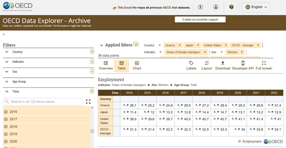
Link to this site: https://stats.oecd.org/index.aspx?queryid=96330
The dataset needed to create the animated line graph is repeated here for you.
Table 3.18: OECD—Percentage of Female Managers
|
Country |
2014 |
2015 |
2016 |
2017 |
2018 |
2019 |
2020 |
2021 |
2022 |
|---|---|---|---|---|---|---|---|---|---|
|
United States |
38.9 |
39.6 |
39.7 |
40.5 |
40.7 |
40.7 |
41.1 |
41.4 |
41.0 |
|
Greece |
28.1 |
25.2 |
24.9 |
29.5 |
27.2 |
28.4 |
29.3 |
29.6 |
31.4 |
|
Japan |
11.4 |
12.0 |
13.3 |
12.8 |
14.4 |
14.7 |
13.1 |
13.2 |
12.9 |
|
OECD Average |
31.3 |
31.4 |
32.2 |
32.3 |
32.5 |
33.3 |
34.0 |
33.6 |
34.1 |
If you want to see all the data captured by the OECD for women managers, please feel free to visit the Excel file: “Case Chapter 3—Share of female managers.”
Case Instructions
- Use Flourish to create an animated line chart from the data listed in Table 3.18.
- Make sure the lines are identified by country.
- Add a title, and add a quote from a woman leader.
- Use the option Publish to share and embed and share the animated graphic URL with the class in the discussion board.
- Be prepared to discuss insights (this will require additional research).
Chapter 3 References
Adamson, K. (2019, Jan 23). Strategy mapping: An essential tool for new academic faculty. Faculty Focus. https://www.facultyfocus.com/articles/faculty-development/strategy-mapping-an-essential-tool-for-new-academic-faculty/
Anscombe, F. J. (1973). Graphs in Statistical Analysis. The American Statistician, 27(1), 17–21.
Bain & Company (2023). Balanced Scorecard fact sheet and statistics. BSC Designer. https://bscdesigner.com/balanced-scorecard-fact-sheet.htm
Business School 101. (2022, Oct 31). Balanced Scorecard (with a step-by-step example) from a business professor [Video]. YouTube. https://youtu.be/W1i59QkU-Ss?si=twvGB4xACP7i2aEL
Center for Teaching Excellence & Innovation. (2022). Effective poster presentation. Johns Hopkins University. https://ctei.jhu.edu/teaching/presentation-strategies/
CPA Strategic Management Accounting. (2023). CPA R. Kaplan explains the Balanced Scorecard. knowledge equity [Video]. YouTube. https://youtu.be/4xXwFwQmRIM?si=OQMBSCsWWRk0hjQZ
de Bruin, L. (2016, Aug 3). Porter’s Five Forces. Business-to-you. https://www.business-to-you.com/porters-five-forces/
de Bruin, L. (2021, Apr 14). Porter’s generic strategies: Differentiation, cost leadership and focus. Business-to-you. https://www.business-to-you.com/porter-generic-strategies-differentiation-cost-leadership-focus/
Delespierre, T., Denormandie, P., Bar-Hen, A., & Josseran, L. (2017). Empirical advances with text mining of electronic health records. BMC Medical Informatics & Decision Making, 17(1), 1–15. ProQuest Database.
Design with Canva. (2022, Dec 22). Flourish + Canva: The perfect match to bring your data to life [Video]. YouTube. https://youtu.be/BpX9JDIhDRw?si=tQ8kT31RVZ3ZehoT
Equity in Athletics Data Analysis. (2023). The tools you need for Equity in Athletics analysis. U.S. Department of Education. https://ope.ed.gov/athletics/#/
Expert Program Management (EPM). (2021, Jun 14). Porter’s Five Forces explained with example [Video]. YouTube. https://youtu.be/q3-8PW72XDQ?si=mQrQN7omBH_crszD
Hall, C. (2022, February 2). Canva acquires Flourish in mission to tell better stories with data. TechCrunch. https://techcrunch.com/2022/02/02/canva-acquires-flourish-in-mission-to-tell-better-stories-with-data/
Holy Cross Crusaders. (2019). Spring 2019 Holy Cross Athletics—Academic highlights. Holy Cross News. https://goholycross.com/news/2019/7/1/211806300.aspx
Hooper, L. (2021, Sept 10). How to use fishbone diagrams to solve complex problems. Venngage. https://venngage.com/blog/fishbone-diagram/
John Carroll University. (2021). Virtual Poster Presentation Guidelines. (2021/22). A Celebration of Scholarship. John Carroll University. https://jcu.edu/sites/default/files/2021-02/Virtual%20Poster%20Presentation%20Guidelines_0.pdf
Kaplan, R. & Norton, D. (1996). Using the Balanced Scorecard as a strategic management system. Harvard Business Review.
Kennedy, J., Ferrier, J., Harbertson, J., Peyrot des Gachons, C. (2006). Analysis of tannins in red wine using multiple methods: Correlation with perceived astringency. American Journal of Enology and Viticulture. Vol 57. 481–485. DOI: 10.5344/ajev.2006.57.4.4.
Lawson, R. A. (Ed.). (2020). Management accounting case book: Cases from the IMA educational case journal. John Wiley & Sons, Incorporated. ProQuest eBook Central Database.
Littlefield, C. (2021). How to make a PowerPoint presentation interactive [Video]. YouTube. https://youtu.be/nWvCvnOZNn4?si=QXAWek1TkRT5X0OU
Marine Training. (2020, Jan 16). How to import data and create graphs in Gapminder [Video]. YouTube. https://youtu.be/mK21HsUI9YE?si=tA7kIcBpD21ENqR5
Mister Simplify. (2023). Quality Function Deployment & the House of Quality—Simplest explanation ever [Video]. YouTube. https://youtu.be/iRMsd-X_e-0?si=FiQlxRZrw40oPOrQ
Mitchell, J. (2021, April 9). Scatter plot in Excel and SPSS Version 27 [Video]. YouTube. https://youtu.be/tIBIZEAV8oo
Modern Work Superheroes. (2022, Nov 9). How to use Word Cloud in Polls for Microsoft Teams [Video]. YouTube. https://youtu.be/KastMzRY-V8?si=rQ8kLRPtLCM6KIX4
Pew Research Center. (2021, January 29). The data on women leaders. Pew Research Center: Facts and trends shaping your world. Pew Research Center. https://www.pewresearch.org/social-trends/fact-sheet/the-data-on-women-leaders
Pluralsight. (2023). State of Cloud 2023: How organizations are maturing in the Cloud. Pluralsight. https://www.pluralsight.com/
Porter, M. (2008). The Five Competitive Forces that shape strategy. Harvard Business Review. https://hbr.org/2008/01/the-five-competitive-forces-that-shape-strategy
SPIE. (2023). Poster presentation guidelines: Create a successful post for presentation at the Conference. SPIE. www.spie.org
United Nations. (2023). United Nations: Department of Economic and Social Affairs, economic analysis. Supplementary graduate indicators (SGI) dataset (2002–2023). United Nations. https://www.un.org/development/desa/dpad/least-developed-country-category/ldc-data-retrieval.html
Vizabi. (2017, April 3). Show your own data. Gapminder.org. https://vizabi.org/tutorials/2017/04/03/show-your-data/
Washington State University. (2022). WSU Athletics Spring 2021 Academic Highlights. Washington State University. https://news.wsu.edu/athletics-spring2021-academic-highlights-infographic/
Zubakov, D., Liu, F., van Zelm, M.C., Vermeulen, J., Oostra, B. A., van Duijn, C. M., Driessen, G. J., van Dongen, J. J. M., Kayser, M., & Langerak, A. W. (2010). Estimating human age from T-cell DNA rearrangements. Current Biology (20)22. https://www.cell.com/action/showPdf?pii=S0960-9822%2810%2901286-8

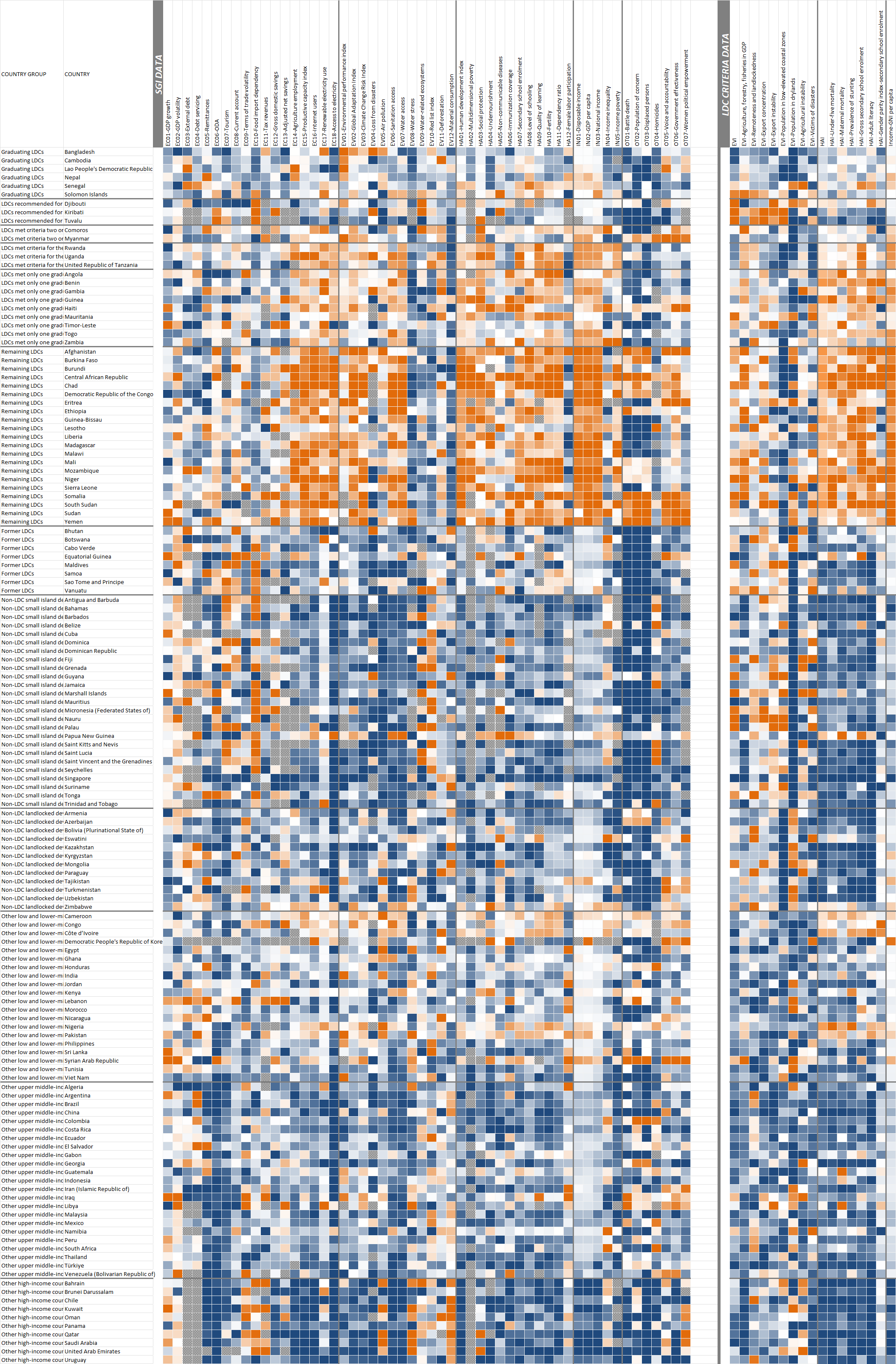