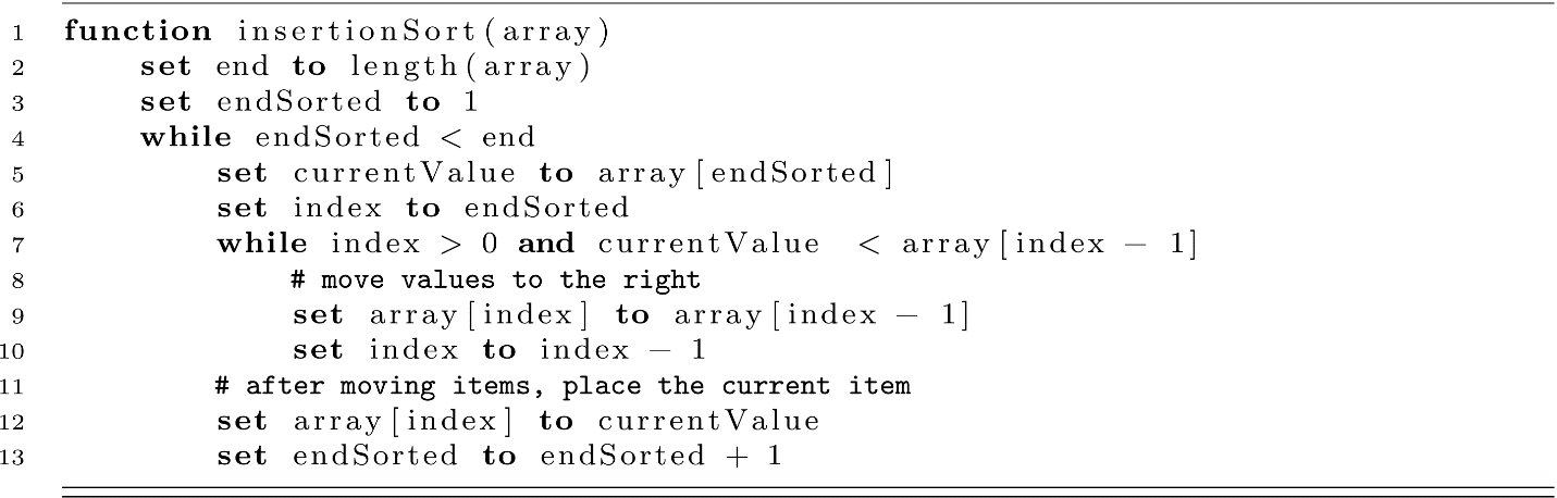
3 Sorting
Learning Objectives
After reading this chapter you will…
- understand the problem of sorting a set of numbers (or letters) in a defined order.
- be able to implement a variety of well-known sorting algorithms.
- be able to evaluate the efficiency and relative advantages of different algorithms given different input cases.
- be able to analyze sorting algorithms to determine their average-case and worst-case time and space complexity.
Introduction
Applying an order to a set of objects is a common general problem in life as well as computing. You may open up your email and see that the most recent emails are at the top of your inbox. Your favorite radio station may have a top-10 ranking of all the new songs based on votes from listeners. You may be asked by a relative to put a shelf of books in alphabetical order by the authors’ names. All these scenarios involve ordering or ranking based on some value. To achieve these goals, some form of sorting algorithm must be used. A key observation is that these sorting problems rely on a specific comparison operator that imposes an ordering (“a” comes before “b” in alphabetical order, and 10 < 12 in numerical order). As a terminology note, alphabetical ordering is also known as lexical, lexicographic, or dictionary ordering. Alphabetical and numerical orderings are usually the most common orderings, but date or calendar ordering is also common.
In this chapter, we will explore several sorting algorithms. Sorting is a classic problem in computer science. These algorithms are classic not because you will often need to write sorting algorithms in your professional life. Rather, sorting offers an easy-to-understand problem with a diverse set of algorithms, making sorting algorithms an excellent starting point for the analysis of algorithms.
To begin our study, let us take a simple example sorting problem and explore a straightforward algorithm to solve it.
An Example Sorting Problem
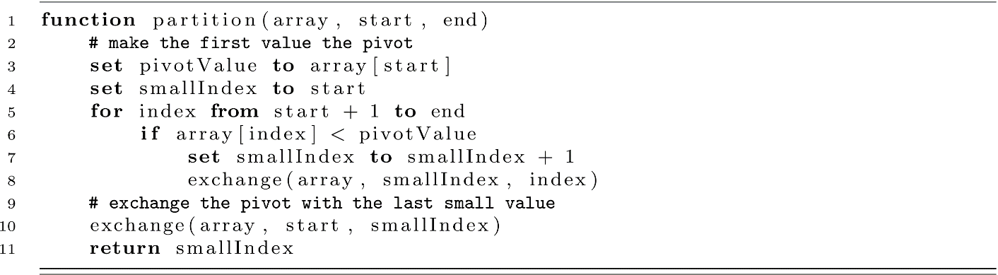
Suppose we are given the following array of 8 values and asked to sort them in increasing order:
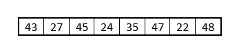
Figure 3.1
How might you write an algorithm to sort these values? Our human mind could easily order these numbers from smallest to largest without much effort. What if we had 20 values? 200? We would quickly get tired and start making mistakes. For these values, the correct ordering is 22, 24, 27, 35, 43, 45, 47, 48. Give yourself some time to think about how you would solve this problem. Don’t consider arrays or indexes or algorithms. Think about doing it just by looking at the numbers. Try it now.
Reflect on how you solved the problem. Did you use your fingers to mark the positions? Did you scan over all the values multiple times? Taking some time to think about your process may help you understand how a computer could solve this problem.
One simple solution would be to move the smallest value in the list to the leftmost position, then attempt to place the next smallest value in the next available position, and so on until reaching the last value in the list. This approach is called Selection Sort.
Selection Sort
Selection Sort is an excellent place to start for algorithm analysis. This sort can be constructed in a very simple way using some bottom-up design principles. We will take this approach and work our way up to a conceptually simple sorting algorithm. Before we get started, let us outline the Selection Sort algorithm. As a reminder, we will use 0-based indexing with arrays:
- Start by considering the first or 0 position of the array.
- Find the index of the smallest value in the array from position 0 to the end.
- Exchange the value in position 0 with the smallest value (using the index of the smallest value).
- Repeat the process by considering position 1 of the array (as the smallest value is now in position 0).
The algorithm works by repeatedly selecting the smallest value in the given range of the array and then placing it in its proper position along the array starting in the first position. With a little thought for our design, we can construct this algorithm in a way that greatly simplifies its logic.
Selection Sort Implementation
Let us start by creating the exchange function. Our exchange function will take an array and two indexes. It will then swap the value in the given positions within the array. For example, exchange(array, 1, 3) will take the value in position 1 and place it in position 3 as well as taking the value in position 3 and placing it in position 1. Let us look at what might happen by calling it on our previous array.
Here is our previous array with indexes added:
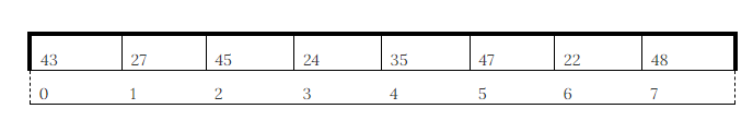
Figure 3.2
After calling exchange(array, 1, 3), we get this:
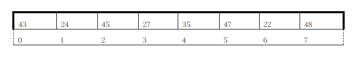
Figure 3.3
This function is the first tool we need to build Selection Sort. Let’s explore one implementation of this function.
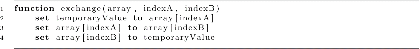
This function will do nothing if the indexes are identical. When we have separate indexes, the corresponding values in the array are exchanged. This evolves the state of the array by switching two values. In this implementation, we do not make any checks to see if an exchange could be made. It may be worth checking if the indexes are identical. It also may be worth checking if the indexes are valid (for example, between 0 and n − 1), but this exercise is left to the reader.
Now we need another tool to help us “select” the next smallest value to put in its correct order. For this task, we need something that is conceptually the same as a findMin function. For our algorithms, we would need to make a few modifications to the regular findMin. The two additions we need to make are as follows: (1) We need to get the index of the smallest value, not just its value. (2) We want to search only within a given range. The last modification will let us choose the smallest value for position 0 and then choose the second smallest value for position 1 (chosen from positions 1 to n − 1).
Let us look at one implementation for this algorithm.
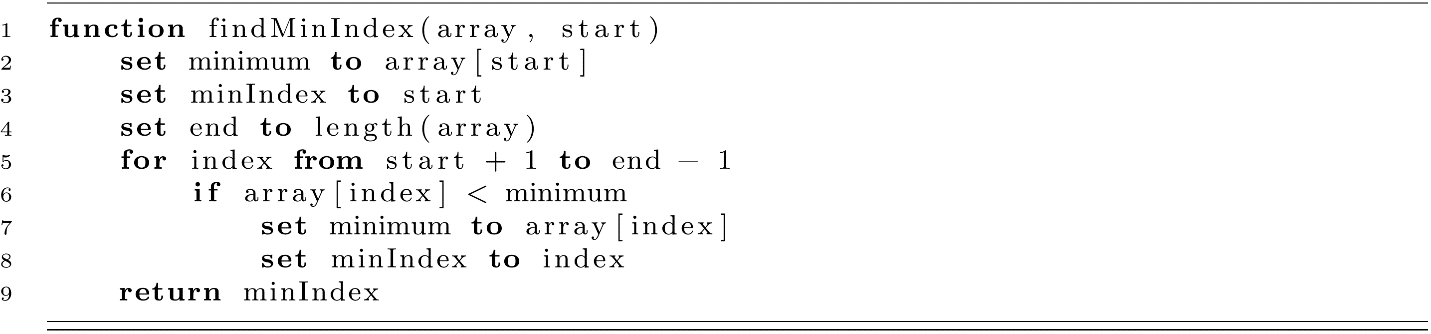
For this algorithm, we can set any start coordinate and find the index of the smallest value from the start to the end of the array. This simple procedure gives us a lot of power, as we will learn.
Now that we have our tools created, we can write Selection Sort. This leads to a simple implementation thanks to the design that decomposed the problem into smaller tasks.

We now have our first sorting algorithm. This algorithm provides a great example of how design impacts the complexity of an implementation. Combining a few simple ideas leads to a powerful new tool. This practice is sometimes called encapsulation. The complexity of the algorithm is encapsulated behind a few functions to provide a simple interface. Mastering this art is the key to becoming a successful computing professional. Amazing things can be built when the foundation is functional, and good design removes a lot of the difficulty of programming. Try to take this lesson to heart. Good design gives us the perspective to program in a manner that is closer to the way we think. Context that improves our ability to think about problems improves our ability to solve problems.
Selection Sort Complexity
It should be clear that the sorting of the array using Selection Sort does not use any extra space other than the original array and a few extra variables. The space complexity of Selection Sort is O(n).
Analyzing the time complexity of Selection Sort is a little trickier. We may already know that the complexity of finding the minimum value from an array of size n is O(n) because we cannot avoid checking every value in the array. We might reason that there is a loop that goes from 1 to n in the algorithm, and our findMinIndex should also be O(n). This idea leads us to think that calling an O(n) function n times would lead to O(n2). Is this correct? How can we be sure? Toward the end of the algorithm’s execution, we are only looking for the minimum value’s index from among 3, 2, or 1 values. This seems close to O(1) or constant time. Calling an O(1) function n times would lead to O(n), right? Practicing this type of reasoning and asking these questions will help develop your algorithm analysis skills. These are both reasonable arguments, and they have helped establish a bound for our algorithm’s complexity. It would be safe to assume that the actual runtime is somewhere between O(n) and O(n2). Let us try to tackle this question more rigorously.
When our algorithm begins, nothing is in sorted order (assume a random ordering). Our index from line 3 of selectionSort starts at 0. Next, findMinIndex searches all n elements from 0 to n − 1. Then we have the smallest value in position 0, and index becomes 1. With index 1, findMinIndex searches n − 1 values from 1 to n − 1. This continues until index becomes n − 1 and the algorithm finishes with all values sorted.
We have the following pattern:
With index at 0 n comparison operations are performed by findMinIndex.
With index at 1 n − 1 comparison operations are performed by findMinIndex.
With index at 2 n − 2 comparison operations are performed by findMinIndex.
…
With index at n − 2 2 comparison operations are performed by findMinIndex.
With index at n − 1 1 comparison operation is performed by findMinIndex.
Our runtime is represented by the sum of all these operations. We could rewrite this in terms of the sum over the number of comparison operations at each step:
n + (n − 1) + (n − 2) + … 3 + 2 + 1.
Can we rewrite this sequence as a function in terms of n to give the true runtime? One way to solve this sequence is as follows:
Let S = n + (n − 1) + (n − 2) + … 3 + 2 + 1.
Multiplying S by 2 gives
2 * S=[n + (n − 1) + (n − 2) + … + 3 + 2 + 1] + [n + (n − 1) + (n − 2) + … + 3 + 2 + 1].
We can rearrange the right-hand side to highlight a useful pattern:
2 * S=[n + (n − 1) + (n − 2) + … + 3 + 2 + 1]
+ [1 + 2 + 3 + … + (n − 2) + (n − 1) + n].
We notice that lining them up with one sequence reversed leads to n terms of n + 1:
2 * S=(n + 1) + (n + 1) + (n + 1) + … + (n + 1) + (n + 1) + (n + 1)
=n * (n + 1).
Now we can divide by two to get an exact function for this summation sequence, which is also known as a variant of the arithmetic series:
S=[n * (n + 1)]/2.
To view it in polynomial terms, we can distribute the n term and move the fraction:
S=(½)*[n2 + n]
=(½) n2 + (½) n.
In Big-O terms, the time complexity of Selection Sort is O(n2). This is also known as quadratic time.
Insertion Sort
Insertion Sort is another classic sorting algorithm. Insertion Sort orders values using a process like organizing books on a bookshelf starting from left to right. Consider the following shelf of unorganized books:
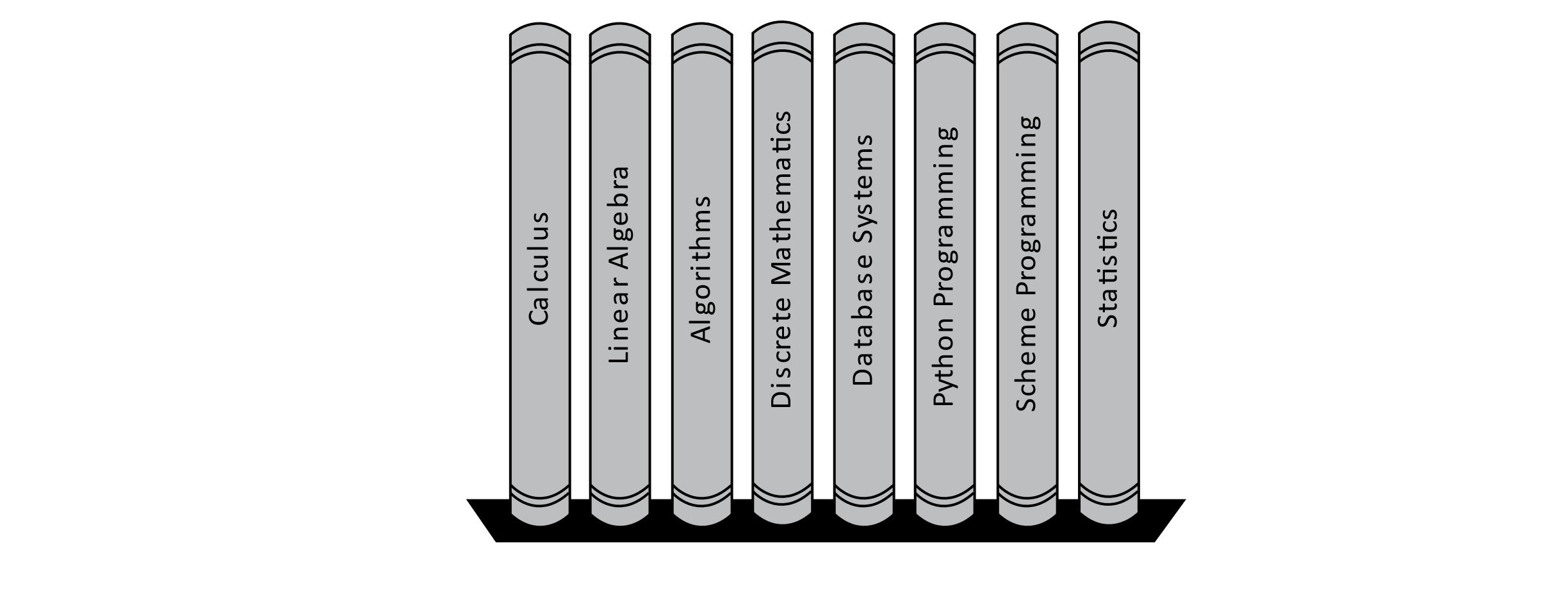
Figure 3.4
Currently, the books are not organized alphabetically. Insertion Sort starts by considering the first book as sorted and placing an imaginary separator between the sorted and unsorted books. The algorithm then considers the first book in the unsorted portion.
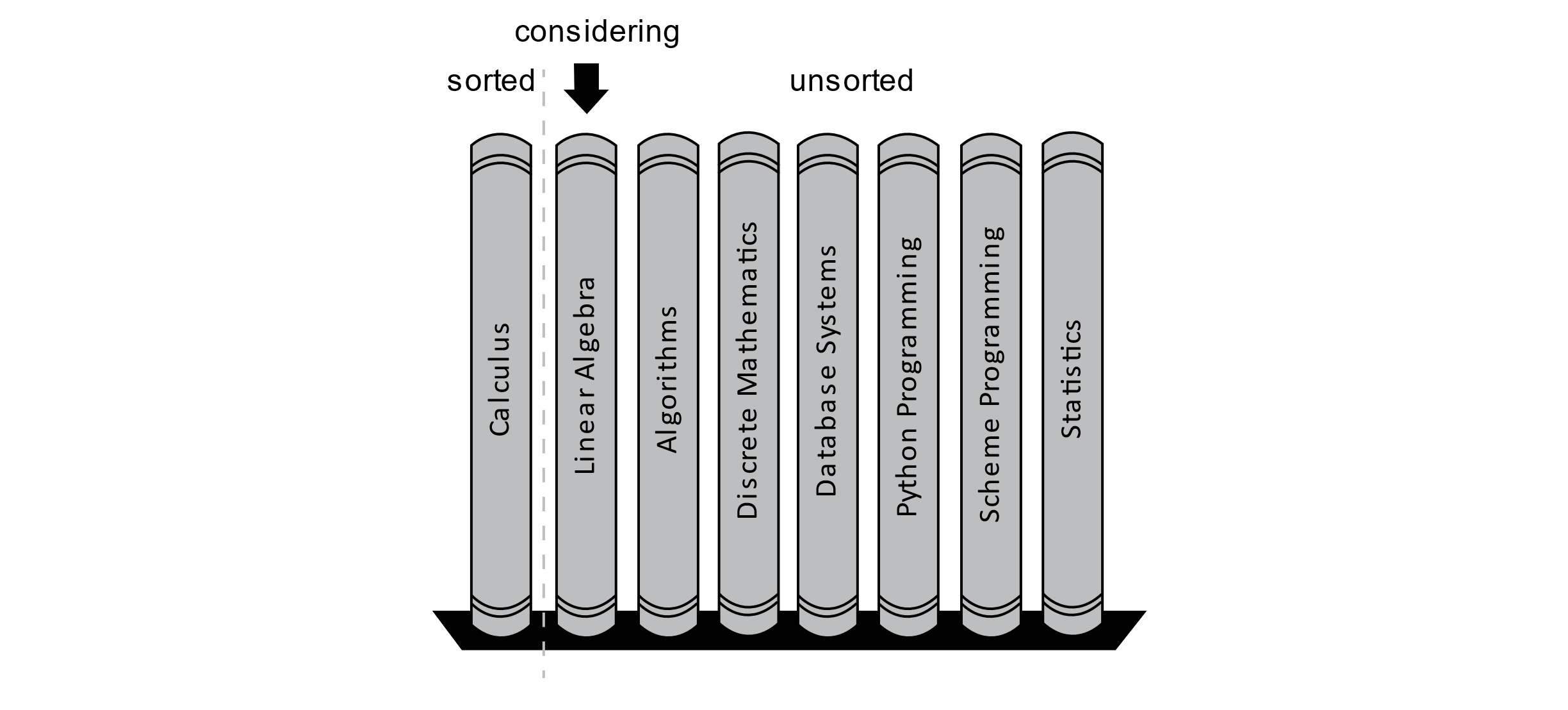
Figure 3.5
According to the image, the algorithm is now considering the book called Linear Algebra. The algorithm will now try to place this new book into its proper position in the sorted section of the bookshelf. The letter “C” comes before “L,” so the book should be placed to the right of the Calculus book, and the algorithm will consider the next book. This state is shown in the following image:
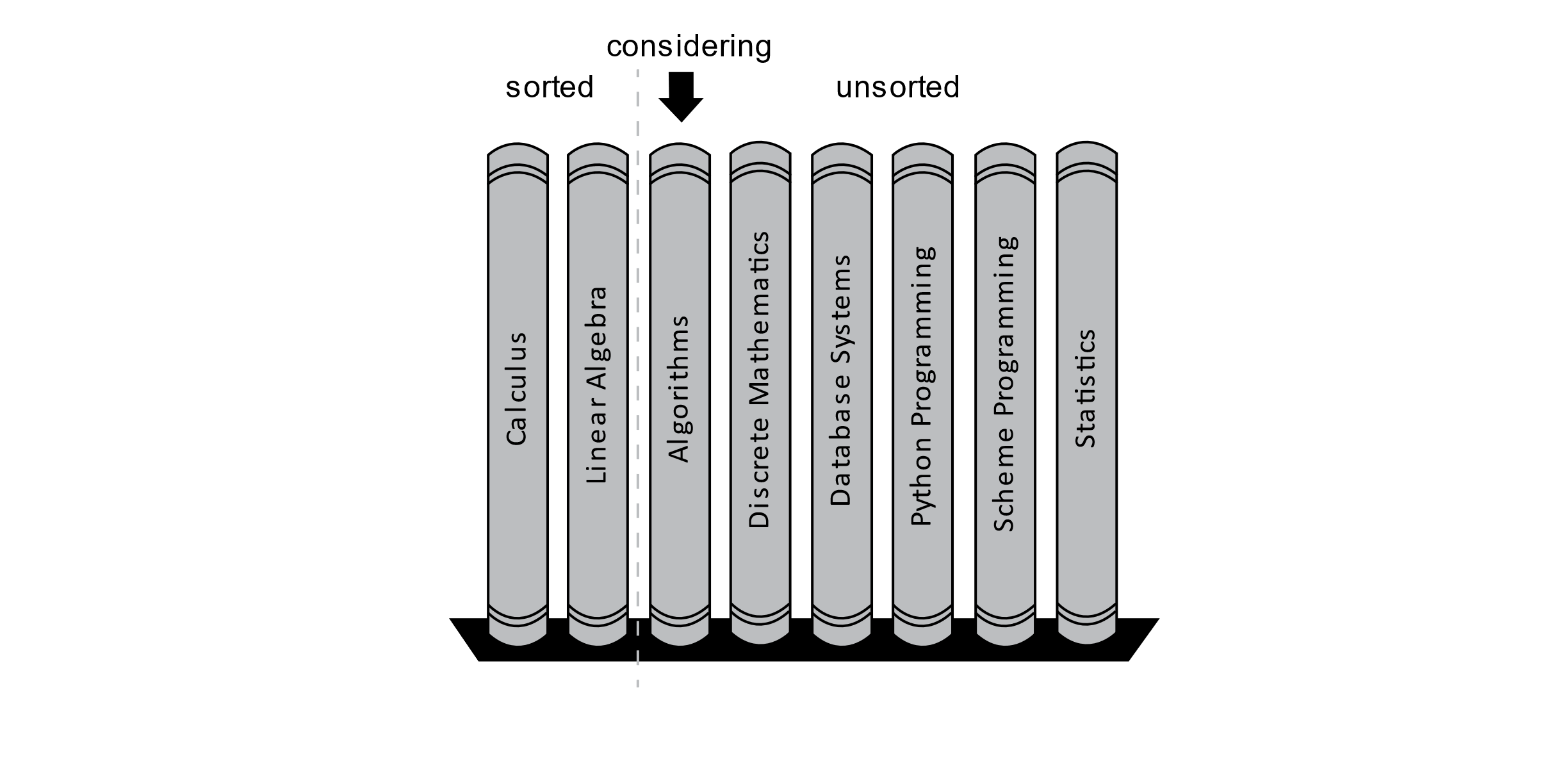
Figure 3.6
Now we consider the Algorithms book. In this case, the Algorithms book should come before both the Calculus and Linear Algebra books, but there is no room on the shelf to just place it there. We must make room by moving the other books over.
The actual process used by the algorithm considers the book immediately to the left of the book under consideration. In this case, the Linear Algebra book should come after the Algorithms book, so the Linear Algebra book is moved over one position to the right. Next, the Calculus book should come after the Algorithms book, and the Calculus book is moved one position to the right. Now there are no other books to reorder, so the Algorithms book is placed in the correct position on the shelf. This situation is highlighted in the following image:
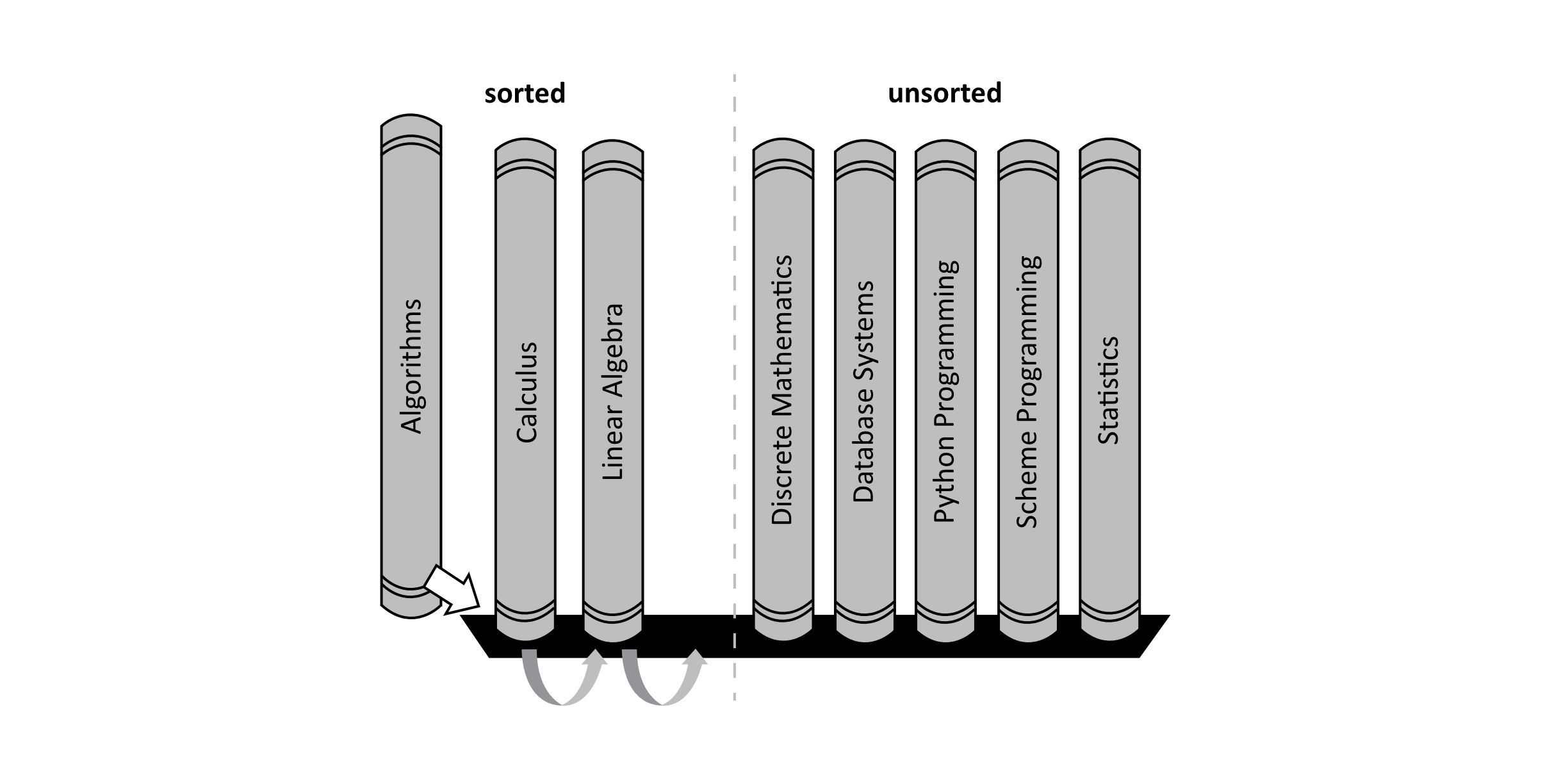
Figure 3.7
After adjusting the position of these books, we have the state displayed below:
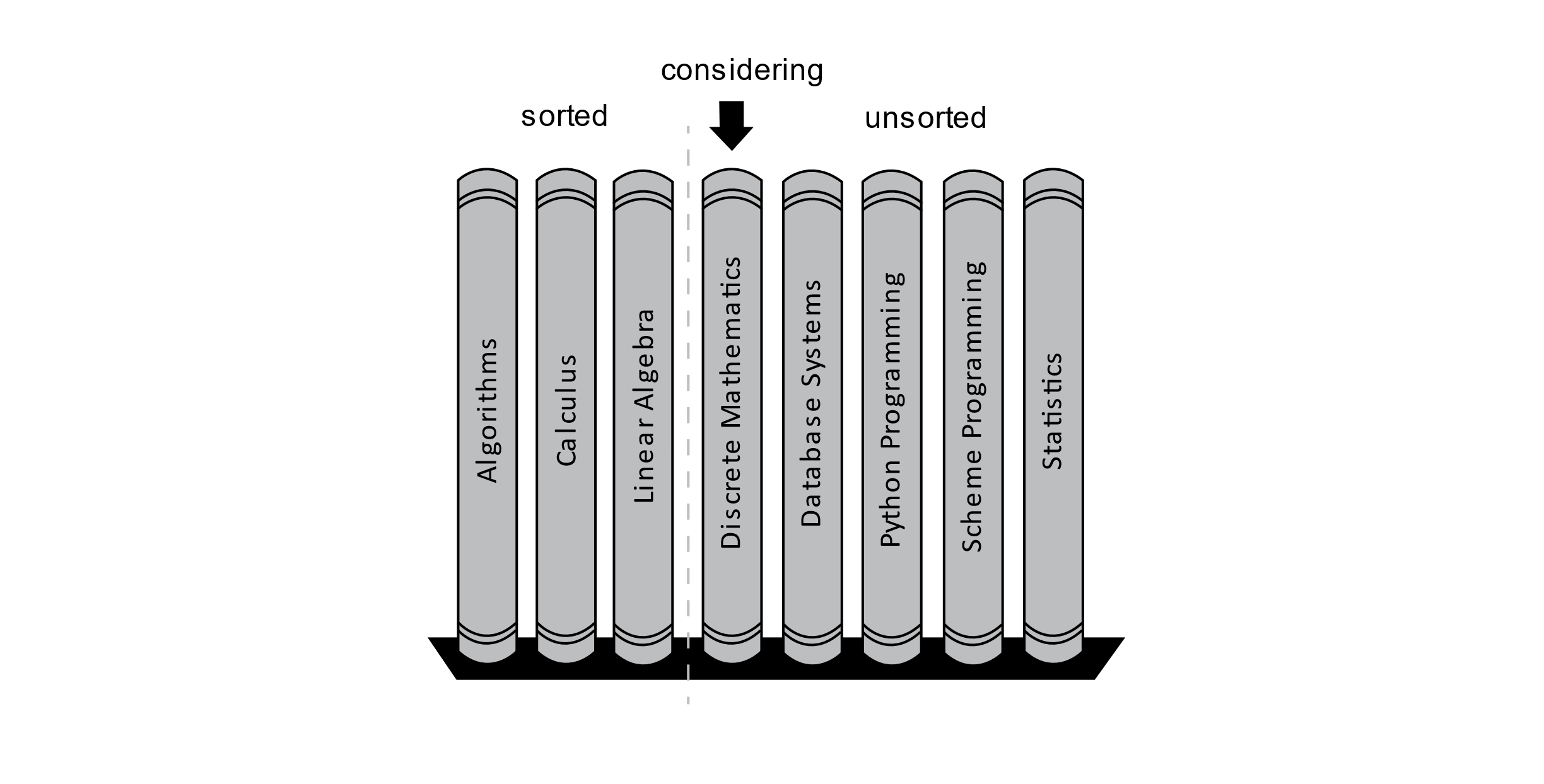
Figure 3.8
Now we consider the textbook on Discrete Mathematics. First, we examine the Linear Algebra book to its left. The Linear Algebra book should go after the Discrete Mathematics book, and it is moved to the right by one position. Now examining the Calculus book informs us that no other sorted books should be after the Discrete Mathematics book. We will now place the Discrete Mathematics book in its correct place after the Calculus book. The Algorithms book at the far left is not even examined. This process is illustrated in the figure below:

Figure 3.9
Once the Discrete Mathematics book is placed in its correct position, the process begins again, considering the next book as shown below:
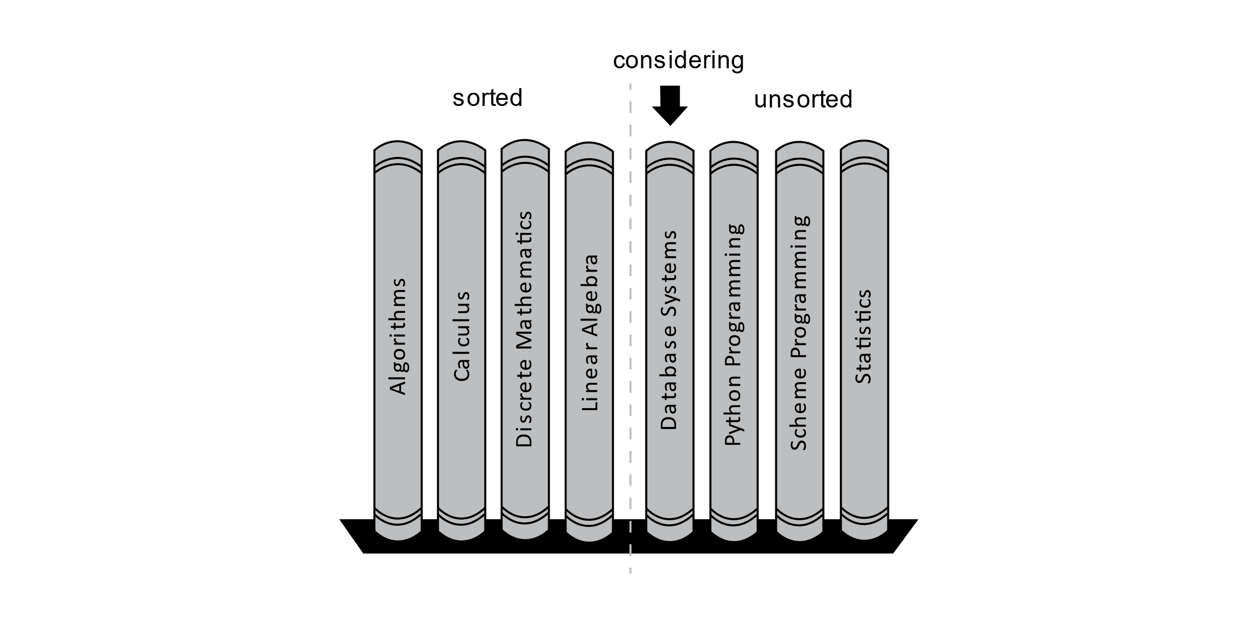
Figure 3.10
This brief illustration should give you an idea of how the Insertion Sort algorithm works. We consider a particular book and then “insert” it into the correct sorted position by moving books that come after it to the right by one position. The sorted portion will grow as we consider each remaining book in the unsorted portion. Finally, the unsorted section of the bookcase will be empty, and all the books will be sorted properly. This example also illustrates that there are other types of ordering. Numerical ordering and alphabetical ordering are probably the most common orderings you will encounter. Date and time ordering are also common, and sorting algorithms will work just as well with these as with other types of orderings.
Insertion Sort Implementation
For our implementation of Insertion Sort, we will only consider arrays of integers as with Selection Sort. Specifically, we will assume that the values of positions in the array are comparable and will lead to the correct ordering. The process will work equally well with alphabetical characters as with numbers provided the relational operators are defined for these and other orderable types. We will examine a way to make comparisons more flexible later in the chapter.
This algorithm relies on careful manipulation of array indexes. Manipulation of array indexes often leads to errors as humans are rarely careful. As always, you are encouraged to test your algorithms using different types of data. Let us test our implementation using the array from before. We will do this by using a trace of an algorithm. A trace is just a way to write out or visualize the sequence of steps in an algorithm. Consider the following array with indexes:
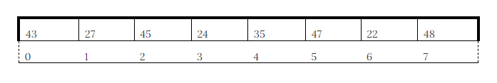
Figure 3.11
The algorithm will start as follows with endSorted set to 1 and end set to 8. Entering the body of the while-loop, we set currentValue to the value 27, and index is set to endSorted, which is 1. The image below gives an illustration of this scenario:
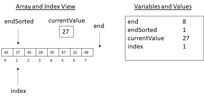
Figure 3.12
We now consider the inner loop of the algorithm. The compound condition of index > 0 and currentValue < array[index − 1] is under consideration. Index is greater than 0, check! This part is true. The value in array[index − 1] is the value at array[1 − 1] or array[0]. This value is 43. Now we consider 27 < 43, which is true. This makes the compound condition of the while-loop true, so we enter the loop. This executes set array[index] to array[index − 1], which copies 43 into position array[index] or array[1]. Next, the last command is executed to update index to index − 1 or 0. This gives us the following state:
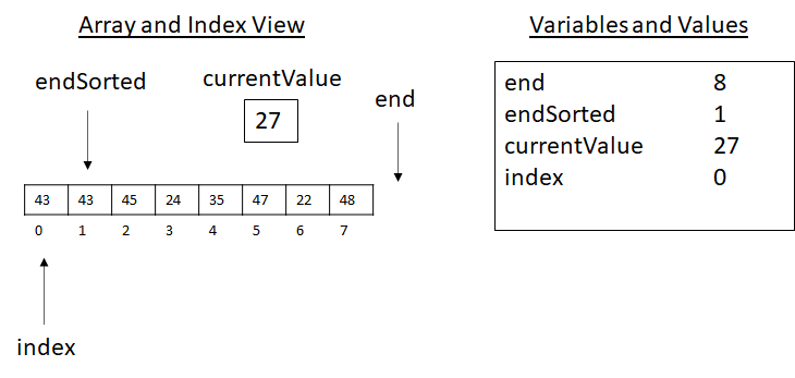
Figure 3.13
You may be thinking, “What about 27? Is it lost?” No, the value of 27 was saved in the currentValue variable. We now loop and check index > 0 and currentValue < array[index − 1] again. This time index > 0 fails with index equal to 0. The algorithm then executes set array[index] to currentValue. This operation places 27 into position 0, providing the correct order. Finally, the endSorted variable is increased by 1 and now points to the next value to consider. At the start of the next loop, after currentValue and index are set, we have the state of execution presented below:
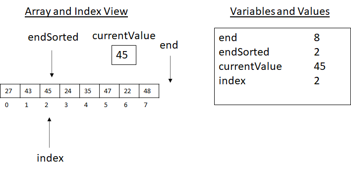
Figure 3.14
Next, the algorithm would check the condition of the inner loop. Here index is greater than 0, but currentValue is not less than array[index − 1], as 45 is not less than 43. Moving over the loop, currentValue is placed back into its original position (line 12), and the indexes are updated at the end of the loop as usual. Moving to the next value to consider, before line 7 we now have the scenarios presented below:
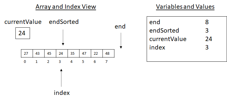
Figure 3.15
From this image, we can imagine what would happen next. The value 24 is smaller than all these values. Let us trace how the algorithm would proceed. As 24 is less than 45, the body will execute copying 45 to the right and updating the index.

Figure 3.16
In the above image, we notice that 24 is less than 43. Therefore, we copy and update our indexes. This gives the following successive states of execution:
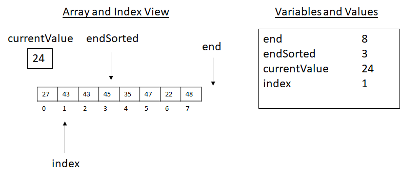
Figure 3.17
Then…

Figure 3.18
Now with index 0, the inner loop’s body will not execute. We will copy the currentValue into the index position and begin the outer loop’s execution again. At the start of the next inner loop, we have the scene below:
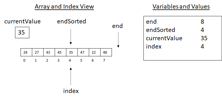
Figure 3.19
These illustrations give you an idea of the execution of the Insertion Sort. These drawings are sometimes called traces. Creating algorithm tracing will give a good idea of how your algorithm is working and will also help you understand if your algorithm is correct or not. From these diagrams, we can infer that the endSorted value will grow to reach the end of the array and all the values will eventually be properly sorted. You should attempt to complete the rest of this trace for practice.
Insertion Sort Complexity
From this example execution, you may have noticed that sometimes Insertion Sort does a lot of work, but other times it seems that very little needs to be done. This observation allows us to consider a different way to analyze algorithms—namely, the best-case time complexity. Before we address this question, let us analyze the worst-case space complexity and the worst-case time complexity of Insertion Sort.
The space complexity of Insertion Sort should be easy to determine. We only need space for the array itself and a few other index- and value-storage variables. This means that our memory usage is O(n) for the array and a small constant number of other values where c << n (a constant much smaller than n). This means our memory usage is bounded by n + c, and we have an O(n) space complexity for Insertion Sort. The memory usage of Insertion Sort takes O(n) for the array itself and O(1) for the other necessary variables. This O(1) memory cost for the indexes and other values is sometimes referred to as the auxiliary memory. It is the extra memory needed for the algorithm to function in addition to the storage cost of the array values themselves. This auxiliary memory could be freed after the algorithm completes while keeping the sorted array intact. We will revisit auxiliary memory later in the chapter.
When considering the time complexity, we are generally interested in the worst-case scenario. When we talk about a “case,” we mean a particular instance of the problem that has some special features that impact the algorithm’s performance. What special features of the way our values are organized might lead to a good or bad case for our algorithm? In what situation would we encounter the absolute largest number of operations? As we observed in our trace, the value 24 resulted in a lot of comparisons and move operations. We continued to check each value and move all the values greater than 24 one space to the right. In contrast, value 45 was nearly in the right place. For 45, we only “moved” it back into the same place from which it came. Take a moment to think about what these observations might mean for our worst-case and best-case analysis.
Let us think about the case of 24 first. Why did 24 require so many operations? Well, it was smaller than all the values that came before it. In a sense, it was “maximally out of place.” Suppose the value 23 came next in the endSorted position. This would require us to move all the other values, including 24, over again to make room for 23 in the first position. What if 22 came next? There may be a pattern developing. We considered some values followed by 24, 23, then 22. These values would lead to a lot of work each time. The original starting order of our previous array was 43, 27, 45, 24, 35, 47, 22, 48. For Insertion Sort, what would be the worst starting order? Or put another way, which starting order would lead to the absolute highest number of comparison and move operations? Take a moment to think about it.
When sorting in increasing order, the worst scenario or Insertion Sort would be an array where all values are in decreasing order. This means that every value being considered for placement is “maximally out of place.” Consider the case where our values were ordered as 48, 47, 45, 43, 35, 27, 24, 22, and we needed to place them in increasing order. The positions of 48 and 47 must be swapped. Next, 45 must move to position 0. Next, 43 moves to position 0 resulting in 3 comparisons and 3 move (or assignment) operations. Then, 35 results in 4 comparisons and 4 move operations to take its place at the front. This process continues for smaller and smaller values that need to be moved all the way to the front of the array.
From this pattern, we see that for this worst-case scenario, the first value considered takes 1 comparison and 1 move operation. The second value requires 2 comparisons and 2 moves. The third takes 3 comparisons and 3 moves, and so on. As the total runtime is the sum of the operations for all the values, we see that a function for the worst-case runtime would look like the following equation. The 2 accounts for an equal number of comparisons and moves:
T(n)=2 * 1 + 2 * 2 + 2 * 3 + 2 * 4 + … 2 * (n − 1).
This can be rewritten as
T(n)=2 * (1 + 2 + 3 + 4 … n − 1).
We see that this function has a growing sum as we saw with Selection Sort. We can substitute this value back into the time equation, T(n):
T(n)=2 * {(½)[n*(n − 1)]}.
The 2 and ½ cancel, leaving
T(n)=n*(n − 1).
Viewing this as a polynomial, we have
T(n)=n2 − n.
This means that our worst-case time complexity is O(n2). This is the same as Selection Sort’s worst-case time complexity.
Best-Case Time Complexity Analysis of Insertion Sort and Selection Sort
Now that we have seen the worst-case scenario, try to imagine the best-case scenario. What feature would that best-case problem instance have for Insertion Sort? In our example trace, we noticed that the value 45 saw 1 comparison and 1 “move,” which simply set 45 back in the same place. The key observation is that 45 was already in its correct position relative to the other values in the sorted portion of the array. Specifically, 45 is larger than the other values in the sorted portion, meaning it is “already sorted.” Suppose we next considered 46. Well, 46 would be larger than 45, which is already larger than the other previous values. This means 46 is already sorted as well, resulting in 1 additional comparison and 1 additional move operation. We now know that the best-case scenario for Insertion Sort is a correctly sorted array.
For our example array, this would be 22, 24, 27, 35, 43, 45, 47, 48. Think about how Insertion Sort would proceed with this array. We first consider 24 with respect to 22. This gives 1 comparison and 1 move operation. Next, we consider 27, adding 1 comparison and 1 move, and so on until we reach 48 at the end of the array. Following this pattern, 2 operations are needed for each of the n − 1 values to the right of 22 in the array. Therefore, we have 2*(n − 1) operations leading to a bound of O(n) operations for the best-case scenario. This means that when the array is already sorted, Insertion Sort will execute in O(n) time. This could be a significant cost savings compared to the O(n2) case.
The fact that Insertion Sort has a best-case time complexity of O(n) and a worst-case time complexity of O(n2) may be hard to interpret. To better understand these features, let us consider the best- and worst-case time complexity of Selection Sort. Suppose that we attempt to sort an array with Selection Sort, and that array is already sorted in increasing order. Selection Sort will begin by finding the minimum value in the array and placing it in the first position. The first value is already in its correct position, but Selection Sort still performs n comparisons and 1 move. The next value is considered, and n − 1 comparisons are executed. This progression leads to another variation of the arithmetic series (n + n − 1 + n − 2 …) leading to O(n2) time complexity. Suppose now that we have the opposite scenario, where the array is sorted in descending order. Selection Sort performs the same. It searches for the minimum and moves it to the first position. Then it searches for the second smallest value, moves it to position 1, and continues with the remaining values. This again leads to O(n2) time complexity. We have now considered the already-sorted array and the reverse-order-sorted array, and both cases led to O(n2) time complexity.
Regardless of the orderings of the input array, Selection Sort always takes O(n2) operations. Depending on the input configuration, Insertion Sort may take O(n2) operations, but in other cases, the time complexity may be closer to O(n). This gives Insertion Sort a definite advantage over Selection Sort in terms of time complexity. You may rightly ask, “How big is this advantage?” Constant factors can be large, after all. The answer is “It depends.” We may wish to ask, “How likely are we to encounter our best-case scenario?” This question may only be answered by making some assumptions about how the algorithms will be used or assumptions about the types of value sets that we will be sorting. Is it likely we will encounter data sets that are nearly sorted? Would it be more likely that the values are in a roughly random order? The answers to these questions will be highly context-dependent. For now, we will only highlight that Insertion Sort has a better best-case time complexity bound than Selection Sort.
Merge Sort
Now we have seen two interesting sorting algorithms for arrays, and we have had a fair amount of experience analyzing the time and space complexity of these algorithms. Both Selection Sort and Insertion Sort have a worst-case time complexity bound of O(n2). In computer science terms, we would say that they are both equivalent in terms of runtime. “But wait! You said Insertion Sort was faster!” Yes, Insertion Sort may occasionally perform better, but it turns out that even the average-case runtime is O(n2). In general, their growth functions are both bounded by O(n2). This fact means that when n is large enough, any minor differences between their actual runtime efficiency will become negligible with respect to the overall time: Graduate Student: “This algorithm is more efficient! It will only take 98 years to complete compared to the 99 years of the other algorithm.” Professor: “I would like to have the problem solved before I pass away. Preferably, before I retire.” This is an extreme example. Often, minor improvements to an algorithm can make a very real impact, especially on real-time systems with small input sizes. On the other hand, reducing the runtime bound by more than a constant factor can have a drastic impact on performance. In this section, we will present Merge Sort, an algorithm that greatly improves on the runtime efficiency of Insertion Sort and Selection Sort.
Description of Merge Sort
Merge Sort uses a recursive strategy to sort a collection of numbers. In simple terms, the algorithm takes two already sorted lists and merges them into one final sorted list. The general strategy of dividing the work into subproblems is sometimes called “divide and conquer.” The algorithm can be specified with a brief description.
To Merge Sort a list, do the following:
- Recursively Merge Sort the first half of the list.
- Recursively Merge Sort the second half of the list.
- Merge the two sorted halves of the list into one list.
Before we investigate the implementation, let us visualize how this might work with our previous array. Suppose we have the following values:

Figure 3.20
Merge Sort would first split the array in half and then make a recursive call on the two subarrays. This would in turn split repeatedly until each array is only a single element. For this example, the process would look something like the image below.

Figure 3.21
Now the algorithm would begin merging each of the individual values into sets of two, then two sets of two into a sorted list of four, and so on. This is illustrated below:

Figure 3.22
The result would be a correctly sorted list. This simple strategy leads to an efficient algorithm, as we will see.
There is one part of the process we have not discussed: the merge process. Let us explore merging at one of the intermediate levels. The example below shows one of the merge steps. The top portion shows conceptually what happens. The bottom portion shows that specific items are moved into specific positions in the new sorted array.

Figure 3.23
To implement Merge Sort, the merge function will be an important part of the algorithm. Let us explore merging with another diagram that more closely resembles our eventual design. At this intermediate step, the data of interest is part of a larger array. These data are composed of two sorted sublists. There are some specific indexes we want to know about. Specifically, they are the start of the first sublist, the end of the first sublist, and the final position of the data representing the end of the data to be merged.

Figure 3.24
Our strategy for merging will be to copy the two sublist sets of values into two temporary storage arrays and then merge them back into the original array. This process is illustrated below:

Figure 3.25
Once the merge process completes, the temporary storage may be freed. This requires some temporary memory usage, but this will be returned to the system once the algorithm completes. Using this approach simplifies the code and makes sure the data are sorted and put back into the original array.
These are the key ideas behind Merge Sort. Now we will examine the implementation.
Merge Sort Implementation
The implementation of algorithms can be tricky. Again, we will use the approach of creating several functions that work together to solve our problem. This approach has several advantages. Mainly, we want to reduce our cognitive load so that thinking about the algorithm becomes easier. We will make fewer errors if we focus on specific components of the implementation in sequence rather than trying to coordinate multiple different ideas in our minds.
We will start with writing the merge function. This function will accept the array and three index values (start of left half, end of left half, and end of data). Notice that for this merge implementation, we use end to refer to the last valid position of the subarray. This use of end is a little different from how we have used it before. Before, we had end specify a value beyond the array (one position beyond the last valid index). Here end will specify the last valid index. The merge function proceeds by copying the data into temporary storage arrays and then merging them back into the original array.
For the copy step, we extend the storage arrays to hold one extra value. This value is known as a sentinel. The sentinel will be a special value representing the highest possible value (or lowest for other orderings). Most programming languages support this as either a MAX or an Infinity construct. Any ordinary value compared to MAX or Infinity will be less than the sentinel (or greater than for MIN or −Infinity with other orderings). In our code, we will use MAX to represent our sentinel construct.
The merge function is presented below:

This function will take a split segment of an array, identified by indexes, and merge the values of the left and right halves in order. This will place their values into their proper sorted order in the original array. Merge is the most complex function that we will write for Merge Sort. This function is complex in a general sense because it relies on the careful manipulation of indexes. This is a very error-prone process that leads to many off-by-one errors. If you forget to add 1 or subtract 1 in a specific place, your algorithm may be completely broken. One advantage of a modular design is that these functions can be tested independently. At this time, we may wish to create some tests for the merge function. This is a good practice, but it is outside of the scope of this text. You are encouraged to write a test of your newly created function with a simple example such as 27, 43, 24, 45 from the diagrams above.
Now that the merge implementation is complete, we will move on to writing the recursive function that will complete Merge Sort. Here we will use the mathematical “floor” function. This is equivalent to integer division in C-like languages or truncation in languages with fixed-size integers.
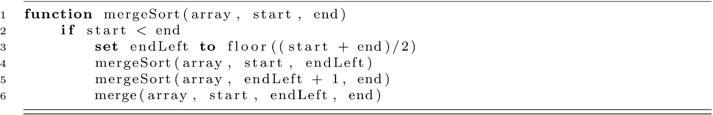
From this implementation, we see that the recursion continues while the start index is less than the end index. Recursion ends once the start and end index have the same value. In other words, our process will continue splitting and splitting the data until it reaches a level of a single-array element. At this point, recursion ends, a single value is sorted by default, and the merging process can begin. This process continues until the final two halves are sorted and merged into their new positions within the starting array, completing the algorithm.
Once more, we have a recursive algorithm requiring some starting values. In cases like these, we should use a wrapper to provide a more user-friendly interface. A wrapper can be constructed as follows:

Merge Sort Complexity
At the beginning of the Merge Sort section, we stated that Merge Sort is indeed faster than Selection Sort and Insertion Sort in terms of worst-case runtime complexity. We will look at how this is possible.
We may begin by trying to figure out the complexity of the merge function. Suppose we have a stretch of n values that need to be merged. They are copied into two storage arrays of size roughly n/2 and then merged back into the array. We could reason that it takes n/2 individual copies for each half of the array. Then another n copies back into the original array. This gives n/2 + n/2 + n total copy operations, giving 2n. This would be O(n) or linear time.
Now that we know merging is O(n) we can start to think about Merge Sort. Thinking about the top-level case at the start of the algorithm, we can set up a function for the time cost of Merge Sort:
T(n)=2*T(n/2) + c*n.
This captures the cost of Merge Sorting the two halves of the array and the merge cost, which we determined would be O(n) or n times some constant c. Substituting this equation into itself for T(n/2) gives the following:
T(n)=2*[2 * T(n/4) + c*n/2] + c*n.
Cleaning things up a little gives the following sequence:
T(n)=2*[2 * T(n/4) + c*(n/2)] + c*n
=4 * T(n/4) + 2*c*(n/2) + c*n
=4 * T(n/4) + c*n + c*n.
As this pattern continues, we will get more and more c*n terms. Instead of continuing the recurrence, we will instead draw a diagram to show how many of these we can expect.

Figure 3.26
Expanding the cost of sorting the two halves, we get the next diagram.

Figure 3.27
As the process continues, the c*n terms start to add up.

Figure 3.28
To determine the complexity though, we need to know how many of these terms to expect. The number of c*n terms is related to the depth of the recursion. We need to know how many times to split the array before arriving at the case where the start index is equal to the end index. In other words, how many times can we split before we reach the single-element level of the array? We just need to solve 1 = n/2k for the value k. Setting k to log2 n solves this equation. Therefore, we have log2 n occurrences of the c*n terms. If we assume that n is a power of 2, the overall time cost gives us T(n) = n*T(1) + log2 n * c * n. For T(1), our wrapper function would make one check and return. We can safely assume that T(1) = c, a small constant. We could then write it as T(n) = n*c + log2 n * c * n, or c*(n * log2 n + n). In Big-O terms, we arrive at O(n log2 n). A consequence of Big-O is that constants are ignored. Logs in any base can be related to each other by a constant factor (log2(n) = log3(n)/log3(2), and note that 1/log3(2) is a constant), so the base is usually dropped in computer science discussions. We can now state the proper worst-case runtime complexity of Merge Sort is O(n log n). It may not be obvious, but this improvement leads to a fundamental improvement over O(n2). For example, at n = 100, n2 = 10000, but n*log2 n is approximately 665, which is less than a tenth of the n2 value. Merge Sort guarantees a runtime bounded by O(n log n), as the best case and worst case are equivalent (much like Selection Sort).
For space complexity, we will need at least enough memory as we have elements of the array. So we need at least O(n) space. Remember that we also needed some temporary storage for copying the subarrays before merging them again. We need the most memory for the case near the end of the algorithm. At this stage, we have two n/2-sized storage arrays in addition to the original array. This leads us to space for the original n values and another n value’s worth of storage for the temporary values. That gives 2*n near the end of the calculation, so overall memory usage seems to be O(n). This is not the whole story though.
Since we are using a recursive algorithm, we may also reason that we need stack space to store the sequence of calls. Each stack frame does not need to hold a copy of the array. Usually, arrays are treated as references. This means that each stack frame is likely small, containing a link to the array’s location and the indexes needed to keep our place in the array. This means that each recursive call will take up a constant amount of memory. The other question we need to address is “How large will the stack of frames grow during execution?” We can expect as many recursive calls as the depth of the treelike structure in the diagrams above. We know now that that depth is approximately log n. Now we have all the pieces to think about the overall space complexity of Merge Sort.
First, we need n values for the original array. Next, we will need another n value for storage in the worst case (near the end of the algorithm). Finally, we can expect the stack to take up around log n stack frames. This gives the following formula using c1 and c2 to account for a small number of extra variables associated with each category (indexes for the temporary arrays, start and end indexes for recursive calls, etc.): S(n) = n + c1*n + c2*log n. This leads to O(2*n + log n), which simplifies to just O(n) in Big-O notation. The overall space complexity of Merge Sort is O(n).
Auxiliary Space and In-Place Sorting
We have now discussed the worst-case space and time complexity of Merge Sort, but an important aspect of Merge Sort still needs to be addressed. All the sorting algorithms we have discussed so far have worst-case space complexity bounds of O(n), meaning they require at most a constant multiple of the size of their input data. As we should know by now, constant values can be large and do make a difference in real-world computing. Another type of memory analysis is useful in practice. This is the issue of auxiliary memory.
It is understood that for sorting we need enough memory to store the input. This means that no sorting algorithm could require less memory than is needed for that storage. A lower bound smaller than n is not possible for sorting. The idea behind auxiliary memory analysis is to remove the implicit storage of the input data from the equation and think about how much “extra” memory is needed.
Let us try to think about auxiliary storage for Selection Sort. We said that Selection Sort only uses the memory needed for the array plus a few extra variables. Removing the array storage, we are left with the “few extra variables” part. It means that a constant number of “auxiliary” variables are needed, leading to an auxiliary space cost of O(1) or constant auxiliary memory usage. Insertion Sort falls into the same category, needing only a few index variables in addition to storage used for the array itself. Insertion Sort has an auxiliary memory cost of O(1).
An algorithm of this kind that requires only a constant amount of extra memory is called an “in-place” algorithm. The algorithm keeps array data as a whole within its original place in memory (even if specific values are rearranged). Historically, this was a very important feature of algorithms when memory was expensive. Both Selection Sort and Insertion Sort are in-place sorting algorithms.
Coming back to Merge Sort, we can roughly estimate the memory usage with this function:
S(n) = n + c1*n + c2*log n.
Now we remove n for the storage of the array to think about the auxiliary memory. That leaves us with c1*n + c2*log n. This means our auxiliary memory usage is bounded by O(n + log n) or just O(n). This means that Merge Sort potentially needs quite a bit of extra memory, and it grows proportionally to the size of the input. This represents the major drawback of Merge Sort. On modern computers, which have sizable memory, the extra memory cost is usually worth the speed up, although the only way to know for sure is to test it on your machine.
Quick Sort
The next sorting algorithm we will consider is called Quick Sort. Quick Sort represents an interesting algorithm whose worst-case time complexity is O(n2). You may be thinking, “n2? We already have an O(n log n) algorithm. I’ll pass, thank you.” Well, hold on. In practice, Quick Sort performs as well as Merge Sort for most cases, but it does much better in terms of auxiliary memory. Let us examine the Quick Sort algorithm and then discuss its complexity. This will lead to a discussion of average-case complexity.
Description of Quick Sort
The general idea of Quick Sort is to choose a pivot key value and move any array element less than the pivot to the left side of the array (for increasing or ascending order). Similarly, any value greater than the pivot should move to the right. Now on either side of the pivot, there are two smaller unsorted portions of the array. This might look something like this: [all numbers less than pivot, the pivot value, all numbers greater than pivot]. Now the pivot is in its correct place, and the higher and lower values have all moved closer to their final positions. The next step recursively sorts these two portions of the array in place. The process of moving values to the left and right of a pivot is called “partitioning” in this context. There are many variations on Quick Sort, and many of them focus on clever ways to choose the pivot. We will focus on a simple version to make the runtime complexity easier to understand.
Quick Sort Implementation
To implement Quick Sort, we will use a few helper functions. We have already seen the first helper function, exchange (above). Next, we will write a partition function that does the job of moving the values of the array on either side of the pivot. Here start is the first and end is the last valid index in the array. For example, end would be n − 1 (rather than n) when partitioning the whole array. This will be important as we recursively sort each subset of values with Quick Sort.
This partition function does the bulk of the work for the algorithm. First, the pivot is assumed to be the first value in the array. The algorithm then places any value less than the pivot on the left of the eventual position of the pivot value. This goal is accomplished using the smallIndex value that holds the position of the last value that was smaller than the pivot. When the loop advances to a position that holds a value smaller than the pivot, the algorithm exchanges the smaller value with the one to the right of smallIndex (the rightmost value considered so far that is smaller than the pivot). Finally, the algorithm exchanges the first value, the pivot, with the small value at smallIndex to put the pivot in its final position, and smallIndex is returned. The final return provides the pivot value’s index for the recursive process that we will examine next.
Using recursion, the remainder of the algorithm is simple to implement. We will recursively sort by first partitioning the values between start and end. By calling partition, we are guaranteed to have the pivot in its correct position in the array. Next, we recursively sort all the remaining values to the left and right of the pivot location. This completes the algorithm, but we may wish to create a nice wrapper for this function to avoid so much index passing.
Quick Sort Complexity
The complexity analysis of Quick Sort is interesting. We know that Quick Sort is a recursive algorithm, so we may reason that its complexity is like Merge Sort. One advantage of Quick Sort is that it is “in place.” There are no copies of the data array, so there should not be any need for extra or “auxiliary” space. Remember though, we do need stack space to handle all those recursive calls and their local index variables. The critical question now is “How many recursive calls can we expect?” This question will determine our runtime complexity and reveal some interesting features of Quick Sort and Big-O analysis in general.
To better understand how this process may work, let’s look at an example using the same array we used with Merge Sort.
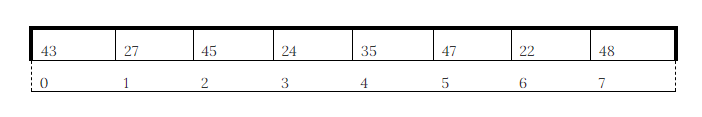
Figure 3.29
Quick Sort would begin by calling partition and setting the pivotValue to 43. The smallIndex would be set to 0. The loop would begin executing with index at 1. Since the value at index (27) is less than the pivot (43), the algorithm would increment smallIndex and exchange it with the value at index. In this case, nothing happens, as the indexes are the same. This is OK. Trying to optimize the small issues would substantially complicate the code. We are striving for understanding right now.

Figure 3.30
With smallIndex updated, execution continues through the loop examining new values. Since 45 is greater than the pivot, the loop simply continues and updates index only.

Figure 3.31
The next value, 24, is smaller than our pivot. This means the algorithm updates smallIndex and exchange values.

Figure 3.32
Now the array is in the following state just before the loop finishes. Next, the index will be incremented, and position 4 will be examined. Notice how smallIndex always points to the rightmost value smaller than the pivot.

Figure 3.33
The partition function will continue this process until index reaches the end of the array. Once the loop has ended, the pivot value at the start position will be exchanged with the value at the smallIndex position.

Figure 3.34
Now the partition function is complete, and the next step in the algorithm is to recursively Quick Sort the left and right partitions. In the figure below, we use startL and endL to mark the start and end of the left array half (and similarly for the right half):
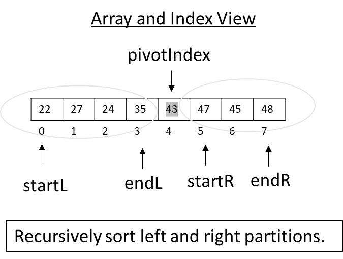
Figure 3.35
Now the process of partitioning would begin again for both sides of the array. You can envision this process growing like a tree with each new partition being broken down into two smaller parts.
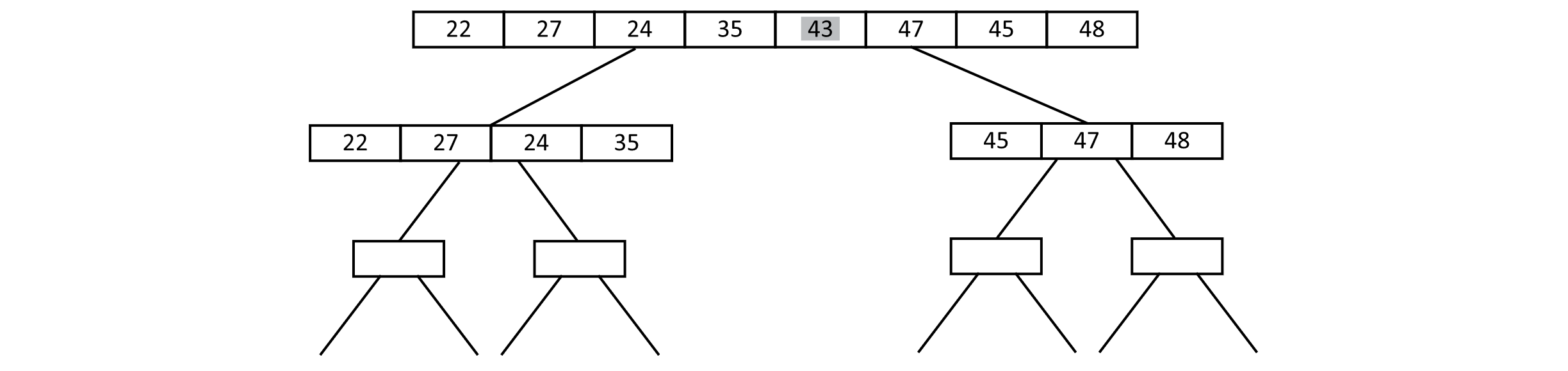
Figure 3.36
Let’s assume that each recursive call to partition breaks the array into roughly equal-size parts. Then the array will be roughly split in half each time, and the tree will appear to be balanced. If this is the case, we can now think about the time complexity of this algorithm. The partition function must visit every value in the array to put it on the correct side of the pivot. This means that partition is O(n). Once the array is split, partition runs on two smaller arrays each of size n/2 as we assumed. For simplicity, we will ignore subtracting 1 for the pivot. This will not change the Big-O complexity. This splitting means that the second level of the tree needs to process two calls to partition with inputs of n/2, so 2(n/2) or n. This reasoning is identical to our analysis of Merge Sort. The time complexity is then determined by the height of this tree. In our analysis of Merge Sort, we determined that a balanced tree has a height of log n. This leads to a runtime complexity of O(n log n).
So if partitioning roughly splits the array in half every time, the time complexity of Quick Sort is O(n log n). That is a big “if” though. Even in this example, we can see that this is not always the case. We said that for simplicity we would just choose the very first value as our pivot. What happens on the very next recursive iteration of Quick Sort for our example?
For the left recursive call, 22 is chosen as the pivot, but it is the smallest value in its partition. This leads to an uneven split. When Quick Sort runs recursively on these parts, the left side is split unevenly, but the right side is split evenly in half.
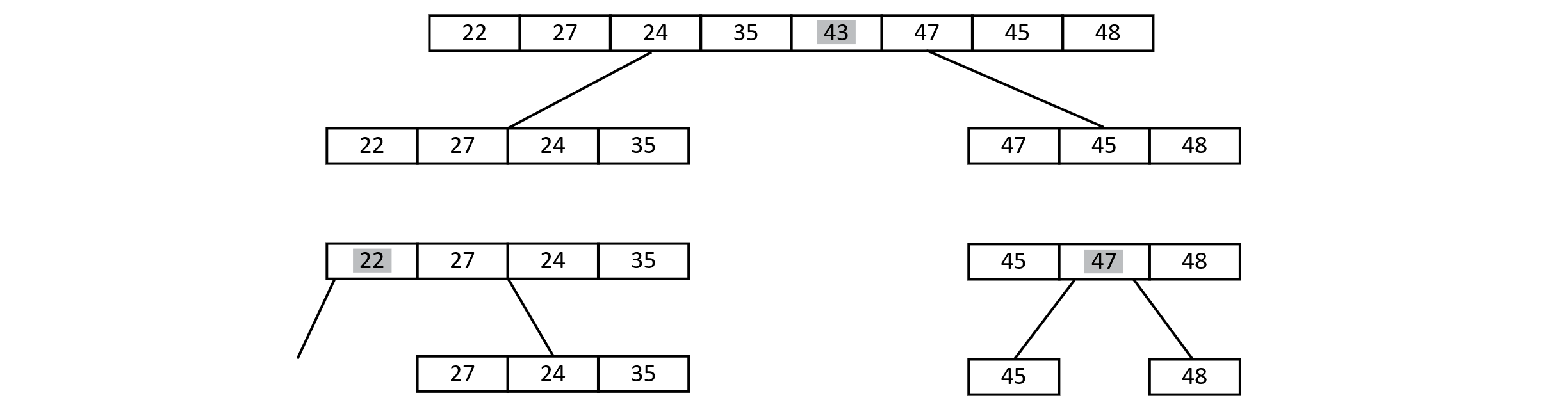
Figure 3.37
The possibility of uneven splits hints that more work might be required. This calls into question our optimistic assumption that the algorithms will split the array evenly every time. This shows that things could get worse. But how bad could it get? Let’s think about the worst-case scenario. We saw that when 22 was the smallest value, there was no left side of the split. What if the values were 22, 24, 27, 35?
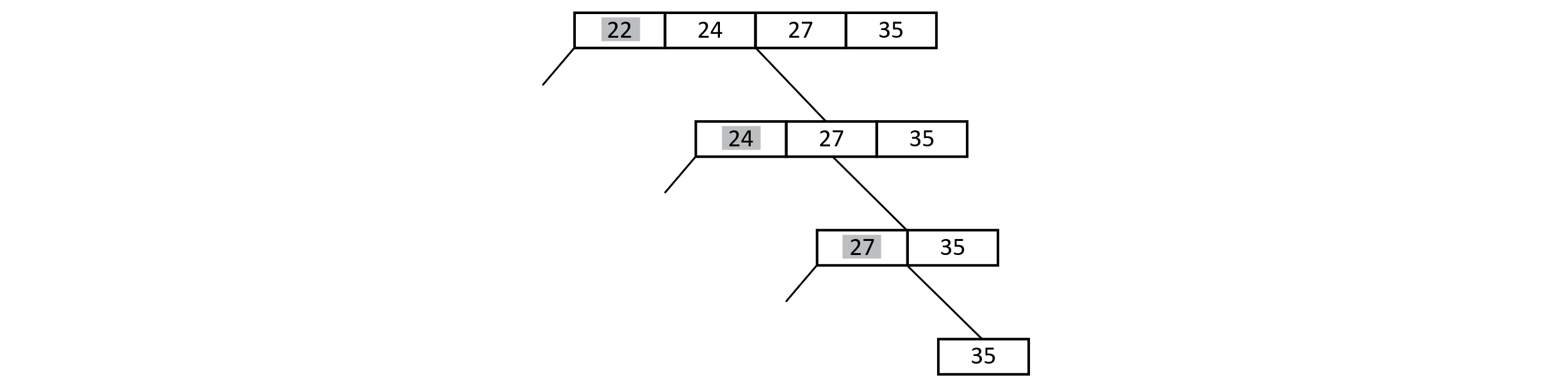
Figure 3.38
This shows an array that is already sorted. Let’s now assume that we have a list that is already sorted, and every time a pivot is chosen, it chooses the smallest value. This means that the partitions that are created are an empty left subset and a right subset that contains all the remaining values minus the pivot. Recursion runs Quick Sort on the remaining n − 1 values. This process would produce a very uneven tree. First, we run partition on n elements, then n − 1 elements, then n − 2, and so on.
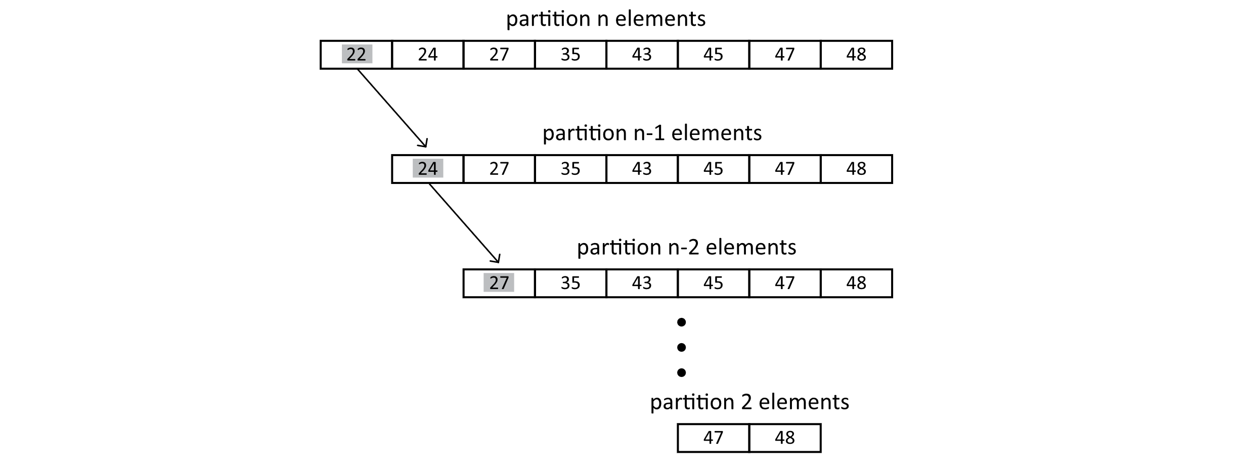
Figure 3.39
This process produces a progression that looks like our analysis of Insertion Sort but in reverse. We get n + n − 1 + n − 2 + … 3 + 2. This leads to a complexity of O(n2). This worst-case runtime complexity is O(n2). You may be thinking that “quick” is not a great name for an algorithm with a quadratic runtime. Well, this is not the full story either. In practice, Quick Sort is very fast. It is comparable to Merge Sort in many real-world settings, and it has the advantage of being an “in-place” sorting algorithm. Let’s next explore some of these ideas and try to understand why Quick Sort is a great and highly used algorithm in practice even with a worst-case complexity of O(n2).
Average-Case Time Complexity
We now know that bad choices of the pivot can lead to poor performance. Consider the example Quick Sort execution above. The first pivot of 43 was near the middle, but 22 was a bad choice in the second iteration. The choice of 47 on the right side of the second iteration was a good choice. Let us assume that the values to be sorted are randomly distributed. This means that the probability of choosing the worst pivot should be 1/n. The probability of choosing the worst pivot twice in a row would be 1/n * 1/(n − 1). This probability is shrinking rapidly.
Here is another way to think about it. The idea of repeatedly choosing a bad pivot by chance is the same as encountering an already sorted array by chance. So the already sorted order is one ordering out of all possible orderings. How many possible orderings exist? Well, in our example we have 8 values. We can choose any of the 8 as the first value. Once the first value is chosen, we can choose any of the remaining 7 values for the second value. This means that for the first two values, we already have 8*7 choices. Continuing this process, we get 8*7*6*5*4*3*2*1. There is a special mathematical function for this called factorial. We represent factorial with an exclamation point (!). So we say that there are 8! or 8 factorial possible orderings for our 8 values. That is a total of 40,320 possible orderings with just 8 values! That means that the probability of encountering by chance an already sorted list of 8 values is 1/8! or 1/40,320, which is 0.00002480158. Now imagine the perfectly reasonable task of sorting 100 values. The value of 100! is greater than the estimated number of atoms in the universe! This makes the probability of paying the high cost of O(n2) extremely unlikely for even relatively small arrays.
To think about the average-case complexity, we need to consider the complexity across all cases. We could reason that making the absolute best choice for a pivot is just as unlikely as making the absolute worst choice. This means that the vast majority of cases will be somewhere in the middle. Researchers have studied Quick Sort and determined that the average complexity is O(n log n). We won’t try to formally prove the average case, but we will provide some intuition for why this might be. Sequences of bad choices for a pivot are unlikely. When a pivot is chosen that partitions the array unevenly, one part is smaller than the other. The smaller subset will then terminate more quickly during recursion. The larger part has another chance to choose a decent pivot, moving closer to the case of a balanced partition.
As we mentioned, the choice of pivot can further improve the performance of Quick Sort by working harder to avoid choosing a bad pivot value. Some example extensions are to choose the pivot randomly or to select 3 values from the list and choose the median. These can offer some improvement over choosing the first element as the pivot. Other variations switch to Insertion Sort once the size of the partitions becomes sufficiently small, taking advantage of the fact that small data sets may often be almost sorted, and small partitions can take advantage of CPU cache efficiency. These modifications can help improve the practical measured runtime but do not change the overall Big-O complexity.
Quick Sort Space Complexity
We should also discuss the space complexity for Quick Sort. Quick Sort is an “in-place” sorting algorithm. So we do not require any extra copies of the data. The tricky part about considering the space complexity of Quick Sort is recognizing that it is a recursive algorithm and therefore requires stack space. As with the worst-case time complexity, it is possible that recursive calls to Quick Sort will require stack space proportional to n. This leads to O(n) elements stored in the array and O(n) extra data stored in the stack frames. In the worst case, we have O(n + n) total space, which is just O(n). Of the total space, we need O(n) auxiliary space for stack data during the recursive execution of the algorithm. This scenario is unlikely though. The average case leads to O(n + log n) space if our recursion only reaches a depth of log n rather than n. This is still just O(n) space complexity, but the auxiliary space is now only O(log n).
Exercises
- Create a set of tools to generate random arrays of values for different sizes in your language of choice. These can be used to test your sorting algorithms. Some useful functions and capabilities are provided below.
- Include functions to generate random arrays of a given size up to 10,000.
- Include functions to print the first 5 numbers or the entire array.
- Provide parameters to control the range of values.
- Provide functions to generate already sorted or reverse sorted arrays.
- Explore your programming language’s time functionality to be able to measure sorting performance in terms of the time taken to complete the sort.
- Consider creating functions to repeatedly run an algorithm and record the average sorting time.
- Implement Selection Sort and Insertion Sort in your language of choice. Using randomly generated array data, try to find the number of values where Insertion Sort begins to improve on Selection Sort. Remember to repeat the sorting several times to calculate an average time.
- Implement Merge Sort and repeat the analysis for Merge Sort and Insertion Sort. For what n does Merge Sort begin to substantially improve on Insertion Sort? Or does it seem to improve at all?
- Implement Quick Sort in your language of choice. Next, determine the time for sorting 100 values that are already sorted using Quick Sort (complete the 1.d exercise). Next, randomly generate 1,000 arrays of size 100 and sort them while calculating the runtime. Are any as slow as Quick Sort on the sorted array? If so, how many? If not, what is the closest time?
References
JaJa, Joseph. “A Perspective on Quicksort.” Computing in Science & Engineering 2, no. 1 (2000): 43–49.
